Central banking in twenty-five drawings

Every drawing uses the same two colours for meaning. Navy marks the ordinary path, and crimson marks the object under study. Look at the drawing first. Then read the text, which says what the drawing claims, and the equation, which says it precisely. The last paragraph of each entry says where the idea stops working.

Lecture 1 · Central bank communication

The first lecture treats communication as a tool of policy. Words move expectations only when people notice them and believe them. The drawings follow that idea from a speech to a household, and then to the institutions that make the words credible.

The communication path

A ribbon flows from a central bank building, bends upward and reaches an investor, a firm and a household — A ribbon leaves the central bank, bends the expected path of rates, and reaches three audiences. An investor, a firm and a household each receive it differently.

A central bank speaks to many audiences at once, and each hears the same message in its own way. An investor watching the yield curve may react within minutes. A firm may change its prices at the next review. A household may not notice the message at all. The words are identical, but the updates are not. Communication is therefore an economic input with uneven effects, and it works only through people who notice it and believe it.

\[\Delta \mathbb{E}_i[\pi] = a_i \, c_i \, m\]

Here \(m\) is the news in the message about future inflation. The term \(a_i\) equals one if audience \(i\) noticed the message and zero if it did not, and \(c_i\), between zero and one, is the weight \(i\) gives to what the central bank says. \(\Delta \mathbb{E}_i[\pi]\) is the resulting change in \(i\)'s expected inflation.

The product is a simplification. Attention and trust are not fixed traits. They change with the news, the speaker and the stakes, so the same audience can respond strongly to one speech and ignore the next.

Anchored expectations

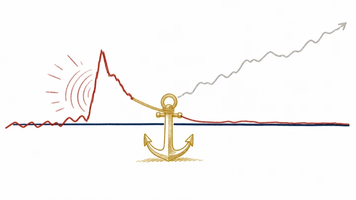
A crimson inflation line jumps after a shock and is pulled back to a navy target line by a gold anchor, while a grey line drifts upward — A shock lifts inflation, drawn in crimson. The gold anchor pulls it back to the navy target line. A grey path without the anchor drifts upward and keeps rising.

Credibility works like an anchor. When people trust the target, a burst of inflation changes what they expect only briefly, and inflation soon falls back. Without that trust, last year's inflation becomes next year's expectation, and the shock feeds on itself. A simple rule captures the difference. Expected inflation is a weighted average of the target and of inflation last period.

\[\pi^e_t = \chi \, \pi^* + (1 - \chi) \, \pi_{t-1}\]

Put this into a Phillips curve, \(\pi_t = \pi^e_t + \alpha x_t + \varepsilon_t\), and subtract the target from both sides.

\[\pi_t - \pi^* = (1 - \chi)\,(\pi_{t-1} - \pi^*) + \alpha x_t + \varepsilon_t\]

Here \(\pi^*\) is the target, \(\chi\) is the weight people place on it, \(x_t\) is the output gap and \(\varepsilon_t\) is a cost shock. Any gap between inflation and the target shrinks by the factor \(1 - \chi\) each period. With \(\chi = 0.8\), four-fifths of a shock is gone after one period. With \(\chi = 0.2\), only a fifth is.

An anchor guides how people update their beliefs. It does not freeze them. If the central bank misses its target for long enough, \(\chi\) itself can fall, and the anchor slips.

Risk and uncertainty

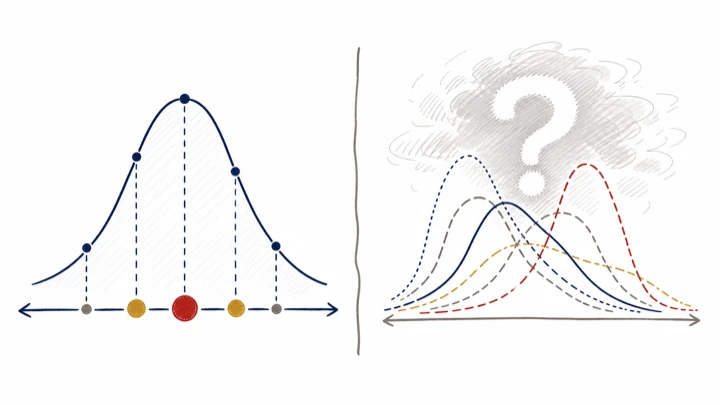
On the left a single bell curve with marked outcomes; on the right several overlapping curves under a grey cloud with a question mark — On the left, one bell curve with known odds and marked outcomes. On the right, several competing curves under a cloud with a question mark.

Risk and uncertainty are different problems. Under risk the policymaker knows the odds. Outcomes vary, but the expected loss can be computed and the tails can be measured. Under uncertainty the odds themselves are in dispute, because economists disagree about which model describes the economy. A precise forecast can then rest on a fragile choice of model.

Under risk the probabilities are known.

\[\mathbb{E}[L] = \sum_{s} p_s \, L_s, \qquad \sum_{s} p_s = 1\]

Under uncertainty there is a set of candidate models instead.

\[Y_{t+h} \sim F_m, \quad m \in \mathcal{M}, \qquad \min_{a} \; \max_{m \in \mathcal{M}} \; \mathbb{E}_m\big[L(a, Y_{t+h})\big]\]

Here \(p_s\) is the probability of state \(s\) and \(L_s\) is the loss in that state. Under uncertainty the outcome \(Y_{t+h}\) follows a distribution \(F_m\) that depends on the model \(m\), and \(\mathcal{M}\) holds the models taken seriously. One cautious response, studied by Hansen and Sargent (2008), chooses the action \(a\) whose worst expected loss across those models is smallest.

The worst-case rule is only one answer. It can be too cautious when the bad model is unlikely, and its result depends on which models are let into \(\mathcal{M}\). Scenarios that show how the decision changes from one model to another are often more useful than a single number.

Independence and accountability

A parliament and a ballot box point to a central bank behind a gold shield; a hand reaches towards the shield; a published report points back to the ballot box — Parliament and the ballot box set the mandate. A gold shield guards the central bank from a hand reaching in. The bank's published report loops back to the voters.

Independence is a division of labour. Elected officials set the objective, and in many countries they also set the inflation target. The central bank then chooses the interest rate that meets it, free from day-to-day political pressure. The shield protects that choice of instrument and nothing more. The bank still has to explain its decisions in reports, minutes and testimony, and those explanations return to the people who set the mandate.

\[i_t = r^* + \pi_t + \phi_\pi \, (\pi_t - \pi^*) + \phi_x \, x_t\]

The government chooses the target \(\pi^*\). The central bank chooses the responses \(\phi_\pi\) and \(\phi_x\), and with them the path of the policy rate \(i_t\). Here \(r^*\) is the neutral real rate and \(x_t\) is the output gap. Taylor (1993) set both responses to one half.

The shield is only as strong as the reporting behind it. Independence lasts when the objective, the forecasts and the mistakes are open to scrutiny. It is harder to defend when a central bank takes on goals that nobody gave it.

Hawk, dove and the trade-off

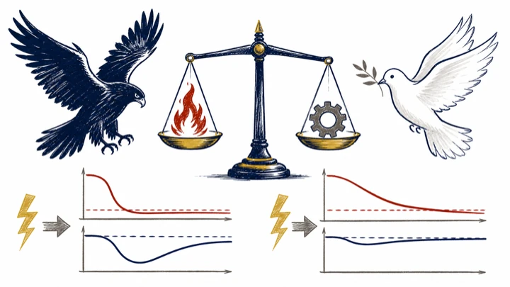
A navy hawk and a white dove either side of a scale holding a flame and a gear; below, two pairs of charts show inflation and output after a shock — A hawk and a dove stand either side of a scale that weighs an inflation flame against an employment gear. Below, the same shock hits twice. Under the hawk, inflation falls fast and output dips deep. Under the dove, inflation falls slowly and output barely moves.

Hawks and doves face the same economy. What separates them is the weight they give to inflation against output. After a cost shock pushes inflation up, a hawk tightens harder and accepts a deeper fall in output to bring inflation back sooner. A dove spreads the adjustment over a longer period. The two labels mark points on a continuum, not two camps.

\[L_t = (y_t - y^e)^2 + \beta \, (\pi_t - \pi^*)^2\]

Take a Phillips curve \(\pi_t = \pi^e_t + \alpha \, (y_t - y^e) + \varepsilon_t\), with expectations given. The output level that minimises the loss each period satisfies

\[y_t - y^e = -\,\alpha \beta \, (\pi_t - \pi^*)\]

Here \(y_t - y^e\) is the gap between output and its efficient level, and \(\beta\) is the weight on inflation. A larger \(\beta\), the hawk, means a larger fall in output for each point of inflation above the target.

The rule assumes the trade-off is known. In practice the slope \(\alpha\), the credibility of the target and the type of shock all change the best response. The same policymaker can rightly sound hawkish in one episode and dovish in the next.

The cat and the ladder

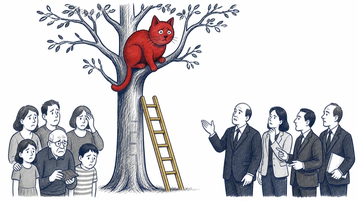
A crimson cat high in a tree, a ladder too short to reach it, worried families on one side and officials on the other — A crimson cat sits high in a tree. The ladder against the trunk is too short to reach it. Worried households watch from one side, and officials argue on the other.

Inflation that has climbed into wage settlements, prices and expectations is like a cat up a tree. It got up quickly. Bringing it down safely takes time, and the job gets harder the longer everyone waits. The short ladder stands for a response that does not match the problem, because the diagnosis is wrong or the tool is too weak. The Phillips curve shows why high expectations make the descent costly.

\[\pi_t = \pi^e_t + \alpha \, x_t + \varepsilon_t \quad\Longrightarrow\quad x_t = \frac{\pi^* - \pi^e_t - \varepsilon_t}{\alpha}\]

To bring inflation \(\pi_t\) back to the target \(\pi^*\) this period, the output gap \(x_t\) must equal the expression on the right. It is negative whenever expected inflation \(\pi^e_t\) sits above the target, so output must fall below potential. A flatter curve, with a smaller \(\alpha\), makes the required fall larger. With \(\pi^e_t\) two points above the target and \(\alpha = 0.5\), the gap must be minus four per cent. With \(\alpha = 0.25\) it must be minus eight.

The equation counts the cost in a single period. A central bank can spread the descent over several years. If its credibility rises along the way, \(\pi^e_t\) falls and less tightening is needed.

Lecture 2 · Measuring expectations

Expectations matter for policy, but nobody observes them directly. The second lecture asks how surveys, market prices and text reveal them, and how to tell a real change in beliefs from a change in the measuring instrument.

Latent beliefs, observable traces

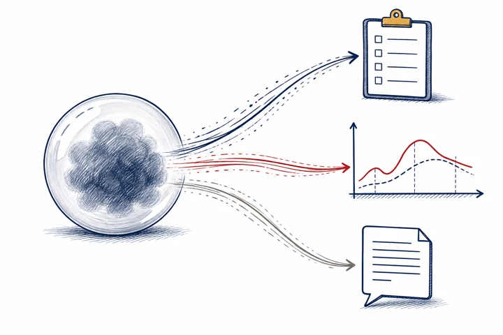
A glass sphere holding a dark cloud sends three bundles of lines to a survey form, a price chart and a written text — A glass sphere holds a dark cloud, the belief itself. Three bundles of lines leave it and arrive at a survey form, a market price chart and a written text.

The object we care about is a belief, such as the inflation a household expects over the next year. A belief leaves no direct record. We see only its traces, in the answer to a survey question, the price of an inflation-linked bond, or the words of a speech or news report. Each trace mixes the belief with features of the instrument that recorded it. Survey wording shifts answers, market prices carry risk premia, and text depends on who wrote it and why.

\[m_{k,t} = \lambda_k \, \theta_t + b_{k,t} + \varepsilon_{k,t}\]

Here \(\theta_t\) is the belief at date \(t\) and \(m_{k,t}\) is what source \(k\) records. Each source has its own scale \(\lambda_k\), its own systematic wedge \(b_{k,t}\), such as a risk premium or a framing effect, and its own noise \(\varepsilon_{k,t}\).

The equation also says what a single measure cannot do. It cannot separate the belief from the wedge. A rise in a market-based measure may mean higher expected inflation or a higher inflation risk premium, and the price alone cannot tell which.

Triangulate the wedges

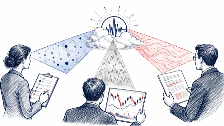
A signal behind clouds is watched by three people through coloured wedges, one with a survey, one with a market screen, one with a marked-up document — A signal hides behind clouds. Three observers look at it through differently coloured wedges. One holds a survey, one a market screen and one a marked-up document.

Three imperfect measures are more useful together than any one alone, because each is distorted in its own way. When surveys, prices and text move at the same time, the shared movement is more likely to be a change in the belief. When they disagree, the disagreement shows where a wedge has moved. Triangulation does not remove the wedges. It puts their differences to work.

\[\Delta m_{k,t} = \lambda_k \, \Delta\theta_t + \Delta b_{k,t} + \Delta\varepsilon_{k,t}, \qquad k = 1, 2, 3\]

If the changes in the wedges \(\Delta b_{k,t}\) are unrelated across the three sources, a movement shared by all of them points to a change in the belief \(\Delta\theta_t\). A shift that appears in one source only points to that source's wedge.

Agreement is evidence, not proof. A bias shared by all three sources can make them agree when the belief has not moved at all.

From beliefs to action

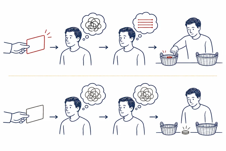
Two rows of the same person; in the top row a crimson card leads to ordered thoughts and a choice, in the bottom row a plain card leaves thoughts tangled and no choice — Two rows show the same person. In the top row a crimson card arrives, the tangled thought becomes ordered, and the person makes a choice. In the bottom row a plain card arrives, the thought stays tangled, and the coin stays on the table.

A measure of beliefs earns its place when it predicts behaviour. Information experiments test this directly. Researchers give one randomly chosen group a piece of information, such as the latest inflation rate, and give a control group nothing new. The difference in beliefs between the two groups is the first stage. The difference in later choices, such as spending or saving, is the reduced form. Their ratio says how far behaviour moves for each unit of belief.

\[\Delta b = \mathbb{E}[\,b \mid Z = 1\,] - \mathbb{E}[\,b \mid Z = 0\,], \qquad \Delta a = \mathbb{E}[\,a \mid Z = 1\,] - \mathbb{E}[\,a \mid Z = 0\,]\]

\[\beta_{\text{IV}} = \frac{\Delta a}{\Delta b}\]

Here \(Z\) equals one for the informed group, \(b\) is the belief and \(a\) is the action. The ratio is the Wald estimator of the effect of beliefs on actions.

The ratio holds only if the information changes behaviour through beliefs and nothing else. If the informed group also feels watched, or guesses the purpose of the study, that condition fails. A small first stage \(\Delta b\) makes the ratio unstable as well.

The calendar average

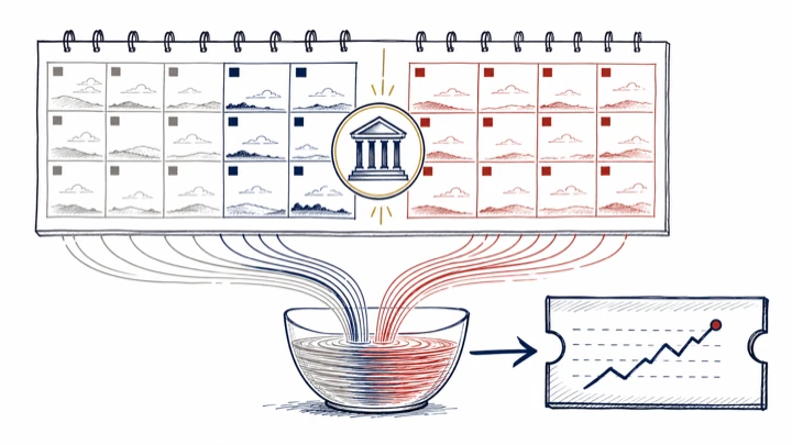
Every day of a monthly calendar pours into a bowl, with the central bank meeting in the middle of the month; the bowl feeds a futures ticket — Every day of the month pours into a single bowl, the days before the meeting and the days after it alike. The mixture sets the price of a futures contract.

Federal funds futures settle on the average policy rate over a calendar month, not on the rate after a meeting. When the meeting falls mid-month, the quote mixes days at the old rate with days at the new one. Reading the quote as the post-meeting rate therefore understates any surprise. The remedy is to undo the averaging.

\[\bar r = \frac{d}{D}\, r_{\text{pre}} + \frac{D - d}{D}\, \mathbb{E}[r_{\text{post}}] \quad\Longrightarrow\quad \mathbb{E}[r_{\text{post}}] = \frac{D\,\bar r - d\, r_{\text{pre}}}{D - d}\]

The surprise on the day of the meeting is then the change in the quote, scaled up.

\[s = \frac{D}{D - d}\,\big(\bar r_{\text{after}} - \bar r_{\text{before}}\big)\]

Here \(D\) is the number of days in the month, \(d\) is the number of days before the decision, \(r_{\text{pre}}\) is the rate on those days and \(\bar r\) is the rate implied by the futures price, equal to 100 minus that price. The factor \(D/(D - d)\) is the adjustment of Kuttner (2001).

Late in the month the factor \(D/(D - d)\) becomes large and magnifies noise, so studies switch to the next month's contract. Two meetings in one month, holidays and month-end effects also need explicit treatment.

Signal inside the window

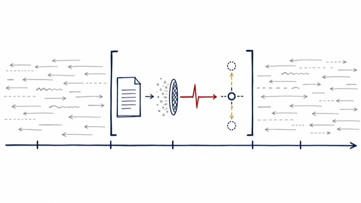
A timeline crowded with grey arrows; inside two brackets a document becomes a single crimson pulse that moves a price up or down — A timeline crowded with grey arrows, news pushing prices in every direction. Inside two brackets, a statement is released and becomes a single crimson pulse that moves the price up or down.

Asset prices move all day for many reasons. To isolate the effect of a policy announcement, researchers look only at a narrow window around it, for example from ten minutes before to twenty minutes after. Little else happens inside that window, so the price change can be attributed to the announcement. Across many announcements, a regression then estimates how strongly a price responds to the surprise.

\[\Delta p_\tau = \beta \, s_\tau + u_\tau\]

Here \(\tau\) indexes announcements, \(\Delta p_\tau\) is the change in an asset price inside the window, \(s_\tau\) is the policy surprise and \(u_\tau\) collects everything else that moved the price in those minutes. A narrow window keeps \(u_\tau\) small.

The window solves a timing problem, not every problem of identification. News released at the same moment enters the window too. A surprise can also carry news about the economy as well as about policy. A higher rate may tell markets that the central bank sees stronger demand than they did, and that information moves prices by itself (Nakamura and Steinsson, 2018).

Signals, wedges and identification

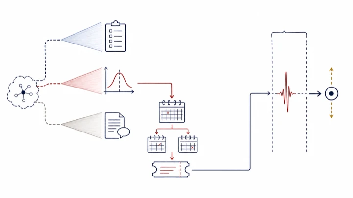
A hidden belief sends dashed lines to a survey, a market and a text; only the market branch continues through calendars and a futures ticket into a narrow window — The whole lecture in one drawing. A hidden belief sends traces to a survey, a market and a text. Only the market branch continues, through the calendar adjustment and a futures contract, into a narrow window where a pulse is measured.

The lecture's two tools answer different questions. Measurement asks what people believe, and surveys, prices and text can all help. Identification asks what caused a change in prices, and only the market branch can answer it. That branch obeys a pricing identity that turns a futures quote into an expected rate, and it trades inside the narrow window.

Measurement links each source to the belief.

\[m_{k,t} = \lambda_k \, \theta_t + b_{k,t} + \varepsilon_{k,t}\]

Identification extracts the surprise from futures prices and estimates its effect inside the window.

\[s_\tau = \frac{D}{D - d}\,\Delta \bar r_\tau, \qquad \Delta p_\tau = \beta \, s_\tau + u_\tau\]

Survey and text evidence can check whether the market surprise means what we think it means. It cannot take the place of that surprise in the regression, because surveys are taken weeks apart and text has no price tied to the policy rate.

Lecture 3 · Monetary policy surprises

Markets price much of a decision before it is announced. The third lecture separates the expected part from the news, splits the news into what it says about today's rate and about the path ahead, and follows it abroad and into markets that are closed when it arrives.

News revises the path

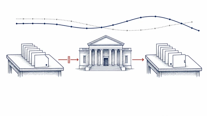
A row of cards on a table passes through a central bank and comes out reordered; above, a dotted and a solid line show expected rates before and after — A row of cards on a table holds the market's schedule of expected rates. After the announcement the same cards stand in a new order. Above, a dotted line shows expected rates before the announcement and a solid navy line shows them after.

Before an announcement, market prices encode an expected rate for every horizon. The announcement can reorder that schedule. Policy news is the revision to the whole path, not only to today's rate. A decision that leaves the current rate unchanged can still move the rate expected a year ahead, and that rate matters for mortgages and company borrowing.

\[S_t(h) = \mathbb{E}_t[\, i_{t+h} \,] - \mathbb{E}_{t^-}[\, i_{t+h} \,]\]

Here \(i_{t+h}\) is the policy rate \(h\) periods ahead, \(t^-\) is the moment just before the announcement and \(t\) the moment just after. The function \(S_t(h)\) traces the news across horizons.

The revision can mix two things. It may reflect a change in how the central bank will react to the economy, or a change in what the central bank knows about the economy. The path alone does not say which.

Expected versus unexpected

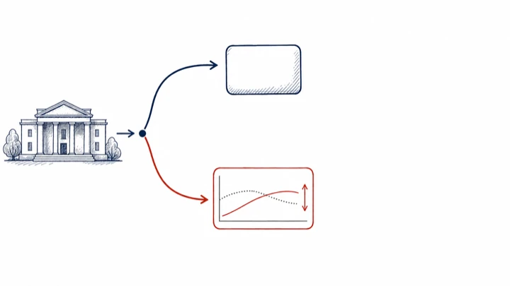
A decision leaves a central bank and splits; a navy branch leads to an empty box, a crimson branch to a chart where two paths separate — A decision leaves the central bank and splits in two. The expected part runs to an empty box, because it is already in prices. The unexpected part runs to a crimson box where the actual and the expected paths separate.

Markets move on surprises, not on decisions. If everyone expected a quarter-point cut and the cut arrives, prices should barely react. The same cut is big news if markets expected no change. Any study of announcement effects has to begin by removing the expected part.

\[A_t = \mathbb{E}_{t^-}[A_t] + u_t, \qquad R_{[t^-,\, t^+]} = \gamma \, u_t + e_t\]

Here \(A_t\) is the announced action, \(\mathbb{E}_{t^-}[A_t]\) is what markets expected just before, and \(u_t\) is the surprise. In an efficient market the return \(R\) over the announcement window responds to \(u_t\), not to the level of \(A_t\).

A surprise is not the same thing as a policy shock. An unexpected rise in rates can mean the central bank has turned more hawkish. It can also mean the bank has seen stronger demand in the data than markets had. The first reading lowers stock prices, and the second can raise them (Jarociński and Karadi, 2020).

Target and path factors

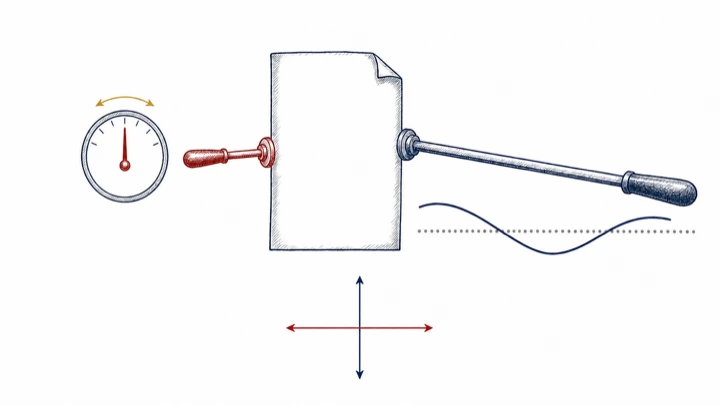
A sheet of paper with a short crimson handle turning a dial and a long navy lever moving a wave; below, two arrows cross at right angles — One announcement, drawn as a sheet of paper, has two handles. A short crimson handle turns a dial, today's rate. A long navy lever moves a wave, the path of rates further ahead. Below, two arrows cross at right angles.

One announcement can move two different things. The target factor captures news about the current policy rate. The path factor captures news about where rates are heading, which mostly comes from guidance and tone. Gürkaynak, Sack and Swanson (2005) showed that two such factors account for the response of money-market futures to Federal Reserve announcements. The path factor had the larger effect on long-term Treasury yields.

\[\Delta f = \Lambda_T \, z_T + \Lambda_P \, z_P + \varepsilon\]

Here \(\Delta f\) is the vector of changes in rate futures across maturities in the announcement window, \(z_T\) and \(z_P\) are the target and path factors, and \(\Lambda_T\) and \(\Lambda_P\) are their loadings. The two factors are rotated so that \(z_P\) has no effect on the current month's rate, which is what makes it a path factor.

The rotation separates two kinds of news. It does not separate a policy action from information about the economy, and either factor can carry either kind.

Global spillover routing

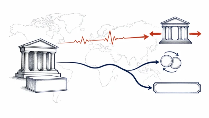
A central bank on a world map sends a crimson pulse to another central bank and a navy route that splits towards two coins and a bond certificate — A central bank on a world map sends two routes abroad. A crimson pulse reaches another central bank. A navy route splits towards the exchange rate, drawn as two coins, and towards bonds.

A policy surprise in one country travels abroad by several routes at once. News about today's rate moves exchange rates and short-term funding costs. News about the path moves long-term yields in many countries through global bond markets. Each asset in each country has its own exposure, which depends on dollar funding, trade links, the duration of its bonds and investors' appetite for risk.

\[R_j = \beta^T_j \, z_T + \beta^P_j \, z_P + \varepsilon_j\]

Here \(R_j\) is the return on asset \(j\) in the window, and \(\beta^T_j\) and \(\beta^P_j\) are its loadings on the target and path factors. Each pair of loadings is estimated asset by asset.

A route on a map is a hypothesis about exposure. The signs and sizes of the loadings have to be estimated. A foreign market that is closed at the time of the announcement has no clean window at all, which is the problem of the next drawing.

The ETF while cash is closed

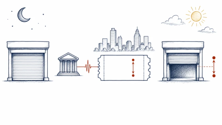
At night a shop shutter is down while a fund ticket in front of a city skyline moves after a policy pulse; in daylight the shutter rises and its jump is compared with the move — At night the home market's shutter is down. A policy pulse reaches a country fund trading in New York, and its price moves. In the morning the shutter rises, and the home market's opening jump is compared with the overnight move.

When a Federal Reserve announcement arrives in the afternoon in New York, the stock markets of Tokyo and Seoul are closed. An exchange-traded fund that holds that country's shares but trades in New York is open, and its price reacts at once. The fund becomes the first place where the news about that market is priced. The home market's jump at the next opening provides a check.

\[R^{\text{ETF}} = \beta_T \, z_T + \beta_P \, z_P + \gamma \, \Delta FX + \varepsilon, \qquad g = \ln P^{\text{open}}_{t+1} - \ln P^{\text{close}}_{t}\]

The fund's return \(R^{\text{ETF}}\) is measured in dollars, so it also carries the change in the exchange rate \(\Delta FX\). The opening gap \(g\) of the home market is the validation. If the fund priced the news correctly, the two should move together.

The fund is an imperfect stand-in. It carries currency moves, its own liquidity and tracking error. The overnight gap also reflects any news that arrives before the home market opens.

The estimand ladder

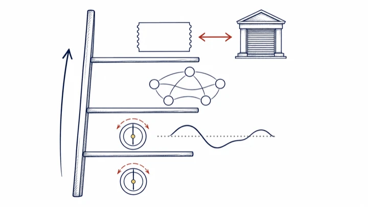
A ladder with four rungs; from the bottom, a dial, a dial with a wave, a network of markets, and a ticket linked to a closed market — A ladder with four rungs. A single dial sits on the bottom rung, a dial and a wave on the next, a network of markets above that, and at the top a traded ticket linked to a closed market.

Each rung of the ladder asks a different question. The bottom rung isolates a rate surprise. The next splits it into target and path news. The third asks how markets around the world respond to each kind of news. The top rung uses traded stand-ins to reach markets that are closed when the news arrives. Climbing adds scope, and it adds assumptions with it.

\[S \;\longrightarrow\; z = (z_T, z_P) \;\longrightarrow\; R_j = \beta_j' z + \varepsilon_j \;\longrightarrow\; R^{\text{ETF}}_j = \beta_j' z + \gamma_j \, \Delta FX_j + \varepsilon_j\]

Each arrow adds something to estimate. The surprise \(S\) becomes a vector of factors \(z\), the factors acquire loadings \(\beta_j\) for every asset \(j\), and the last step replaces a closed market with a traded proxy.

A higher rung is more ambitious, not more credible. Every step needs tighter alignment of clocks, richer data and more controls, and an error made on a low rung is carried up to every rung above it.

Lecture 4 · Communication as text data

Central banks publish more than ever, in statements, minutes, speeches, reports and posts. The fourth lecture asks what can be learned by treating those words as data, and what cannot.

The hidden middle

A document on a podium sends a dashed line past an eye and an ear towards three people and a blank signpost — A document on a podium sends a dashed line towards an audience and a blank signpost. On the way the line passes an eye and an ear, and its middle stretch turns crimson.

Between a publication and a change in behaviour lies a chain of steps that studies often skip. The document has to be seen. It has to be understood. Only then can it change beliefs or decisions. Counting documents, or the words in them, measures only the first step. The empirical task is to measure the steps in the middle.

\[\Delta Y_{i,t} \approx \beta \, \big( P_t \times A_{i,t} \times I_{i,t} \big) + \varepsilon_{i,t}\]

Here \(P_t\) records the publication, \(A_{i,t}\) whether person \(i\) paid attention to it, \(I_{i,t}\) how \(i\) interpreted it, and \(\Delta Y_{i,t}\) the change in \(i\)'s beliefs or behaviour. If \(A_{i,t}\) or \(I_{i,t}\) is zero, the publication has no effect on \(i\).

The product is a teaching device, not an estimated model. It says that an effect needs every step. It does not say how strong each step is, and that is what the data have to show.

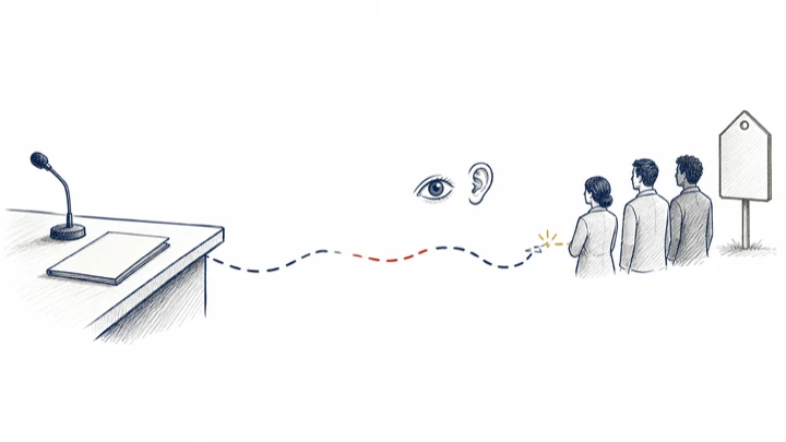
The bundled release

Loose papers and envelopes fly into a single gold folder; on the other side lines burst out towards readers at different distances — Loose papers and envelopes fly into a single gold folder. On the other side, lines burst out towards readers at different distances.

A central bank can publish its documents one at a time or in a single package. Bundling concentrates the material into fewer moments. A large release may become an event that many people notice. It may also overwhelm readers, so that each one reads less of it. The choice trades how many people engage against how deeply each one reads.

\[\text{material per release} = \frac{R}{B}, \qquad \text{attention} = \sum_{b=1}^{B} \text{reach}_b \times \text{depth}_b\]

Here \(R\) documents are grouped into \(B\) releases. Fewer releases put more material into each one. Total attention depends on the reach and the depth of every release, and both can change with the size of the bundle.

Reach and depth have to be measured separately. Page views can show reach. Depth needs reading time, recall or follow-up questions, which are harder to collect.

Interpretation is not approval

A text reaches an ear; a prism in a thought bubble passes the message straight through; below, a gold thumbs up and a crimson thumbs down — A text reaches an ear. Inside a thought bubble, a prism passes the message straight through. Below, one hand gives a gold thumbs up and the other a crimson thumbs down.

Two listeners can decode the same message correctly and react to it in opposite ways. Both hear that rates will stay high for longer. One approves, and the other objects. Comprehension and agreement are separate outcomes. A sentiment score that merges them into one number mistakes disagreement for misunderstanding.

\[C_i \approx 1 \;\not\Longrightarrow\; G_i \approx 1\]

Here \(C_i\) measures how well person \(i\) understood the message, on a scale from zero to one, and \(G_i\) measures how far \(i\) agrees with it on the same scale. Full comprehension does not imply agreement.

A successful message can therefore make a policy clearer and less popular at the same time. That outcome shows the communication worked. It is not a sign that it failed.

A published post competes

A hand releases a navy card into a fast stream of grey cards and speech bubbles while an eye scans the stream — A hand releases a navy card into a fast stream of grey cards and speech bubbles, while an eye scans the stream.

Publishing a post makes it available, not seen. The central bank's message enters a feed crowded with other news, opinion and noise, and the platform decides what reaches each person. Impressions count the chances to see a post. Clicks show that someone chose to open it. Neither shows that the reader understood the message or acted on it.

\[\Pr(\text{act}) = \Pr(\text{see}) \times \Pr(\text{understand} \mid \text{see}) \times \Pr(\text{act} \mid \text{understand})\]

This is the chain rule of probability. A message has to be seen before it is understood and understood before it is acted on, so a small first factor limits everything after it.

Timing, format, the platform's ranking and competing news all shift the first factor. A study that measures only impressions learns about the first step and nothing about the other two.

The disclosure iceberg

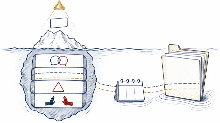
A lamp lights a small card above an iceberg; beneath the water, layers hold debate, a warning triangle and two raised hands; dashed lines run to a calendar and a folder — A lamp lights the small card above the waterline. The larger body lies beneath it, with debate, risks, and votes on both sides. Dashed lines run from the hidden layers to a calendar and a folder that are released later.

The policy statement is the visible tip. Below it lie the minutes, the forecasts, the risk assessments, the alternatives that were discussed, and the votes with any dissents. Markets react within minutes to the statement. The deeper record, published later, explains why the committee acted. More disclosure adds to what the public can know. It does not always add to what the public understands.

\[\frac{\partial \, \text{understanding}}{\partial \, |I_t|} < 0 \quad \text{when } |I_t| \text{ is large}\]

Here \(I_t\) is the information the central bank releases and \(|I_t|\) is its size. Understanding rises with disclosure at first and can fall once the material exceeds the attention readers have.

Depth and accessibility have to be judged separately. A full record serves specialists and accountability, and a short, clear summary serves everyone else. Neither replaces the other.

The mandate translation gate

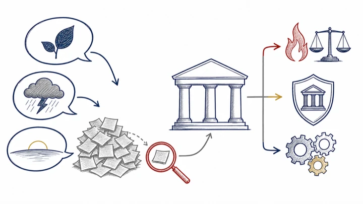
Speech bubbles with a leaf, a storm and a sun on the horizon feed a pile of papers; a magnifying glass picks one; it passes through a central bank and splits towards inflation, financial stability and the economy — Three concerns, drawn as a leaf, a storm cloud and a sun on the horizon, arrive as a pile of papers. A crimson magnifying glass picks out one piece of evidence. It passes through the central bank and splits towards inflation and price stability, the safety of banks, and the working of the economy.

A concern such as climate change enters monetary policy only through a gate, and two questions decide whether it passes. Is the evidence credible? And through which channel does it reach the central bank's mandate? Climate risk can move inflation through food and energy prices and output through damage and disruption. It can also lower the value of collateral, weaken banks and affect the central bank's own operations. Through those channels it is a matter for monetary policy. Outside them it is not.

\[i_t = \phi_\pi \, (\pi_t - \pi^*) + \phi_y \, x_t + \cdots, \qquad \frac{\partial i_t}{\partial c_t} = \phi_\pi \, \frac{\partial \pi_t}{\partial c_t} + \phi_y \, \frac{\partial x_t}{\partial c_t}\]

Here \(c_t\) is a climate shock. In the rule it affects the policy rate \(i_t\) only through inflation \(\pi_t\) and the output gap \(x_t\), the variables the mandate names.

Mentioning climate in a speech is not the same as adding a new objective, and the equation draws the line between the two. A shock that changes inflation or output is inside the mandate. A goal pursued for its own sake needs a mandate that elected officials have given.

The readability toolbox

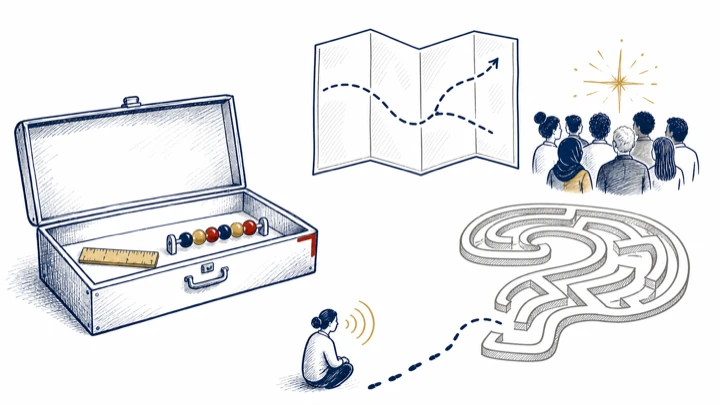
An open toolbox with a ruler and syllable beads; around it a map with a winding path, an audience under a gold star, and a maze shaped like a question mark that a listener sets out to cross — An open toolbox holds a ruler and a string of syllable beads. Around it lie what the tools cannot measure. There is a map with a winding path, an audience under a gold star, and a maze in the shape of a question mark that one listener sets out to cross.

Readability formulas measure the surface of a text. They count words per sentence and syllables per word, so they catch long sentences and long words. They cannot tell whether an argument is clear, whether a key term is understood, or whether the reader already knows enough to follow it. Those questions need tests of comprehension with real readers.

\[\text{reading ease} = 206.835 - 1.015 \left( \frac{\text{words}}{\text{sentences}} \right) - 84.6 \left( \frac{\text{syllables}}{\text{words}} \right)\]

This is the formula of Flesch (1948). Higher scores mean easier text, and scores between 60 and 70 are usually read as plain English.

Use the score as a first check. A short sentence can still hide a hard idea, and a long one can be clear to its audience. Understanding has to be tested through interpretation, recall or tasks, not inferred from word counts.

References

Flesch, R. (1948). A new readability yardstick. Journal of Applied Psychology, 32(3), 221–233.
Gürkaynak, R. S., Sack, B. and Swanson, E. T. (2005). Do actions speak louder than words? The response of asset prices to monetary policy actions and statements. International Journal of Central Banking, 1(1), 55–93.
Hansen, L. P. and Sargent, T. J. (2008). Robustness. Princeton University Press.
Jarociński, M. and Karadi, P. (2020). Deconstructing monetary policy surprises: the role of information shocks. American Economic Journal: Macroeconomics, 12(2), 1–43.
Kuttner, K. N. (2001). Monetary policy surprises and interest rates: evidence from the Fed funds futures market. Journal of Monetary Economics, 47(3), 523–544.
Nakamura, E. and Steinsson, J. (2018). High-frequency identification of monetary non-neutrality: the information effect. Quarterly Journal of Economics, 133(3), 1283–1330.
Taylor, J. B. (1993). Discretion versus policy rules in practice. Carnegie-Rochester Conference Series on Public Policy, 39, 195–214.