Probability & Statistics · Lecture 1 of 5
Probability theory
What can happen, and how should information change what we believe?
1 Describe→2 Condition→3 Learn
- 1Probability theoryWhat can happen, and how does information change it?
- 2Data, variables & momentsHow do measurements vary?
- 3StatisticsWhat can one sample tell us about a population?
- 4Time seriesWhat changes when observations depend on their past?
- 5Causal inferenceWhich comparison identifies an effect?
Developed from Ian Crawford’s lecture material. Notes, slides and PDF: fatih.ai/probabilityandstatistics
Opening question
A cyclist tests positive. How likely is it that the cyclist uses EPO?
A hypothetical cycling population and an imperfect test:
Your estimateVote now and keep your answer. Part 3 calculates it.
Why start here
Economists read signals backwards all the time: a test result, a credit score, a qualification. Today builds the rules that make that reading exact.
Lecture 1 · The route
Describe uncertainty, condition on information, learn from evidence
Part 1
Describe: events and their probabilities
What exactly could happen, and how do we give events probabilities that are consistent with one another?
sample spaceeventaxiomsunion rule
Notes 1.1
Part 2
Condition: how information changes a probability
When we learn that one event has happened, how should the probability of another change?
conditional probabilityproduct ruletotal probability
Notes 1.2
Part 3
Learn: independence and Bayes’ rule
When does information leave a probability unchanged, and how should evidence change what we believe?
independenceBayes’ rulepriorposteriorbase rate
Notes 1.3
By the end of this lecture you can
- Write the sample space and events for an experiment, and derive the complement and union rules from the axioms.
- Calculate a conditional probability as a share within the information event, keeping track of which way it runs.
- Combine group rates by total probability, and check whether two events are independent.
- Update a prior with Bayes’ rule, and explain why a positive EPO test means about 57%, not 90%.
1
Part 1 of 3
Describe: events and their probabilities
What exactly could happen, and how do we give events probabilities that are consistent with one another?
Key terms
sample spaceeventaxiomsunion ruleWhy it matters
Every economic question about risk, from becoming unemployed to a loan default, starts by stating exactly which outcome is uncertain. The axioms keep the probabilities we attach consistent with one another, whatever the weights.
In this part
- 1.1.1–3Outcomes, events and set operations
- 1.1.4The axioms and the complement rule
- 1.1.5The union rule
- ▶Animation: where each term of the union rule comes from
1.1.1–3Outcomes and events
Events are sets of outcomes, so “not”, “and”, “or” are set operations
Definition
Sample space and events
An outcome ω is one possible result; the sample space Ω collects them all. An event A⊆Ω is the set of outcomes that make a statement true.
| Statement | Event | One die: B even, C prime |
|---|---|---|
| not B | Bc | {1,3,5} |
| B and C | B∩C | {2} |
| B or C | B∪C | {2,3,4,5,6} |
“Or” is inclusive. Events are disjoint when A∩B=∅.
A picture of “and”, “or” and “not”
1.1.4The axioms
Three axioms fix how probabilities combine, not what they are
Definition
The axioms of probability
- P(A)≥0 for every event: no negative mass.
- P(Ω)=1: the total is fixed.
- Disjoint events add: P(⋃iAi)=∑iP(Ai) for pairwise disjoint Ai.
Worked example a fair and a loaded die
Fair: P(even)=3×61=21. Loaded, 0.1 on faces 1–5 and 0.5 on face 6: P(even)=0.1+0.1+0.5=0.7. Both satisfy the axioms.
Key formula Result (1)
Complement rule
In words A and Ac are disjoint and fill Ω, so their probabilities add to 1.
Common mistake
Probability zero is not impossibility: one exact bulb lifetime can have probability 0 without being impossible.
1.1.5Adding probabilities
Adding two events counts their overlap twice
Key formula Result (2)
Union rule
In words add both, then remove the overlap counted twice.
Needs any two events; when they are disjoint the last term is zero.
Disjointness lets you add; overlap must be subtracted once.
Check
Fair die, B even, C prime. What is P(B∪C)?
Answer
63+63−61=65. The plain sum, 1, counts the face 2 twice.
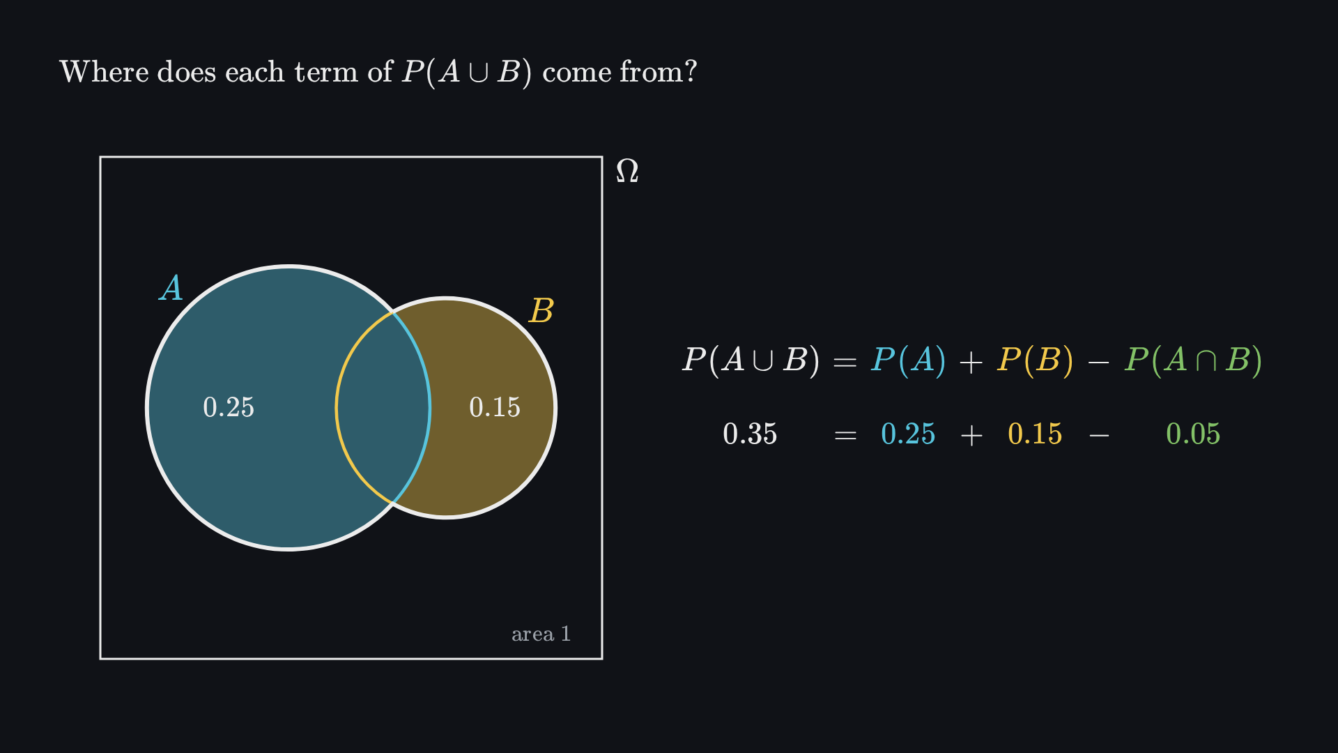
Before it plays Play to see each term of P(A∪B)=P(A)+P(B)−P(A∩B) come from the picture. The areas are drawn to scale, so every probability is an area.
2
Part 2 of 3
Condition: how information changes a probability
When we learn that one event has happened, how should the probability of another change?
Key terms
conditional probabilityproduct ruletotal probabilitySo far a model (Ω,F,P), three axioms, and the complement and union rules.
Why it matters
Economic information usually arrives as rates within groups: defect rates per production line, unemployment among graduates, default among borrowers with a given score. Answering the question asked needs the right reference group, and recombining groups needs their sizes as weights.
In this part
- 1.2.1Two children: information and the reference group
- 1.2.2Conditional probability: restrict, then rescale
- ▶Animation: why conditioning divides by the probability of the information
- 1.2.3Reversing the condition
- 1.2.4Total probability: a weighted average of group rates
- ▶Animation: total probability as a weighted average
1.2.1Information changes the question
Learning something changes the group in which we calculate
Two children, each a boy or a girl with probability 21, independently, older child first:
Ω={(b,b),(b,g),(g,b),(g,g)}Each family has probability 41. Let A be “two boys” and B “at least one boy”.
Predict first
We learn that B is true. Are two boys now more or less likely than 41?
Answer
More: (g,g) is ruled out, so three equally likely families remain and P(A∣B)=31.
No family changes. What changes is the group in which we calculate the share.
1.2.2The definition
Conditional probability: restrict to B, then rescale B to one
Key formula Definition (3)
Conditional probability
In words the share of B that also lies in A: conditional probability.
Needs P(B)>0.
- Restrict to B: only A∩B survives.
- Rescale by 1/P(B): the new total is 1.
Key formula Identity (4)
Product rule
In words the definition turned around: a share of a share.
Worked example
P(B)=0.6 and P(A∩B)=0.1, so
P(A∣B)=0.60.1=61,P(Ac∣B)=65.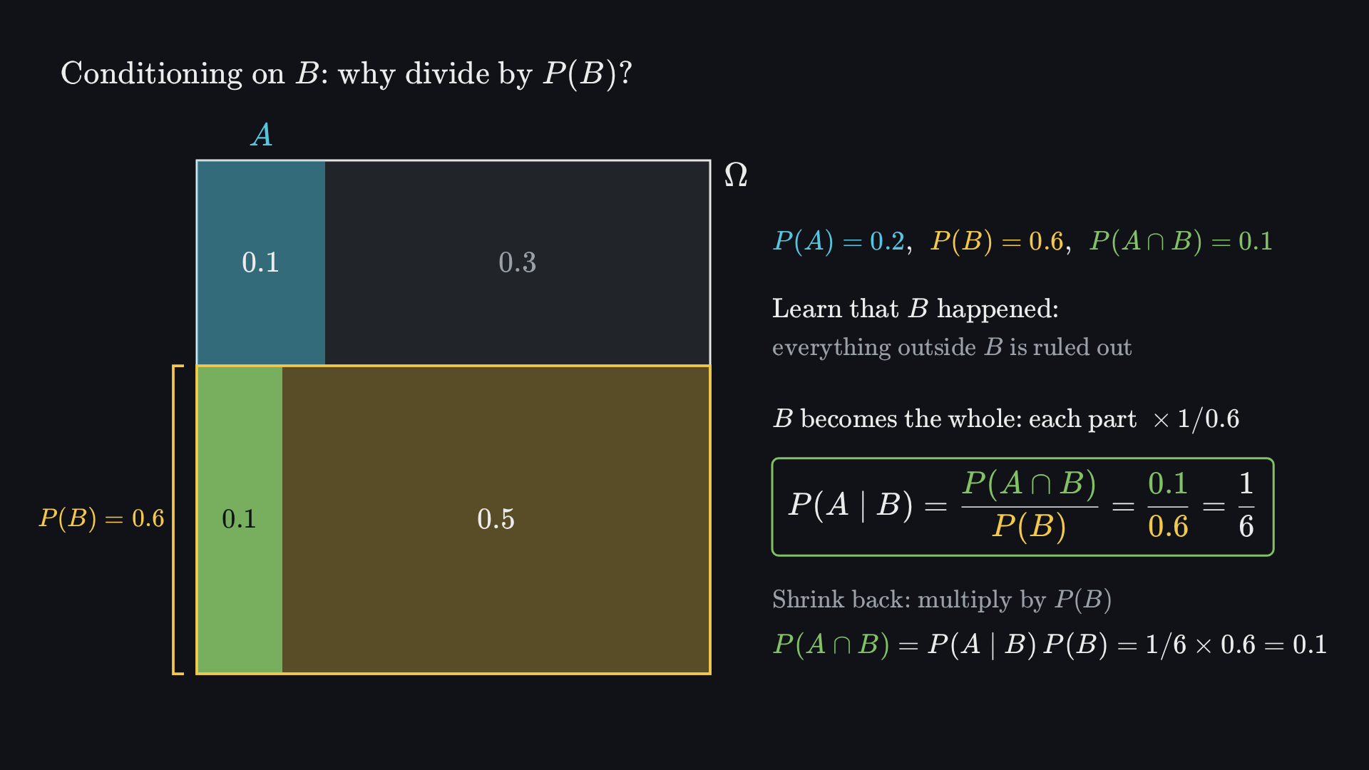
Before it plays Before playing, predict: when B is stretched to fill the whole square, what share of it will the overlap fill?
1.2.3Direction matters
Reversing the condition changes the denominator
| B | Bc | Total | |
|---|---|---|---|
| A | 10 | 10 | 20 |
| Ac | 50 | 30 | 80 |
| Total | 60 | 40 | 100 |
Within column B: P(A∣B)=10/60=61
Within row A: P(B∣A)=10/20=21
Common mistake
Treating P(A∣B) and P(B∣A) as the same number. They share a numerator, P(A∩B), but divide by different groups.
Reading claims
“Most students are Democrats” does not say that most Democrats are students. Read the condition first: it names the group you divide by.
1.2.4Recovering the whole
Total probability weights each group’s rate by the group’s size
Key formula Result (5)
Law of total probability
In words each group’s rate times its share, added over the groups.
Needs groups Bi that cover Ω without overlap (a partition), each P(Bi)>0.
Worked example the 100 cases
P(A)=61(0.6)+41(0.4)=0.1+0.1=0.2
Check
Line 1 makes 40% of items with defect rate 0.05; line 2 makes 60% with rate 0.10. What share of all items is defective?
Answer
0.05(0.4)+0.10(0.6)=0.02+0.06=0.08. The plain average, 0.075, would treat the lines as equal in size.
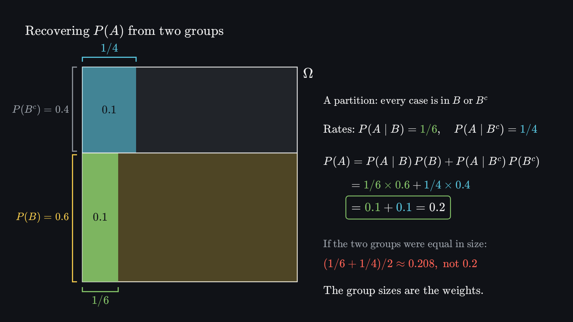
Before it plays Before playing, predict: is P(A) the plain average of the two group rates, 1/6 and 1/4?
3
Part 3 of 3
Learn: independence and Bayes’ rule
When does information leave a probability unchanged, and how should evidence change what we believe?
Key terms
independenceBayes’ rulepriorposteriorbase rateSo far conditioning restricts to the information event and rescales it; total probability weights group rates by group sizes.
Why it matters
Decisions rest on imperfect signals read backwards: a positive drug test, a credit score, rare evidence in court. Bayes’ rule makes the reversal exact, and independence says when information is irrelevant and when probabilities may be multiplied.
In this part
- 1.3.1Independence: an unchanged share
- ▶Animation: independence as an unchanged share
- 1.3.2Bayes’ rule: one joint probability, two directions
- 1.3.3The EPO test, step by step
- ▶Animation: every number in the posterior
- 1.3.4–5Base rates and the Sally Clark case
1.3.1Independence
Independent events: learning B leaves the probability of A unchanged
Key formula Definition (6)
Independence
In words equivalently P(A∣B)=P(A): the share of A inside B equals its share overall.
Needs the equivalent form needs P(B)>0.
Independence is a fact about overlap, checked by comparing probabilities.
Worked example
P(A)=0.30 and P(B)=0.40. Independence needs P(A∩B)=0.30×0.40=0.12, and then
P(A∣B)=0.400.12=0.30=P(A).Common mistake
Disjoint is not independent. If A∩B=∅ and both have positive probability, learning B rules A out: P(A∣B)=0=P(A).
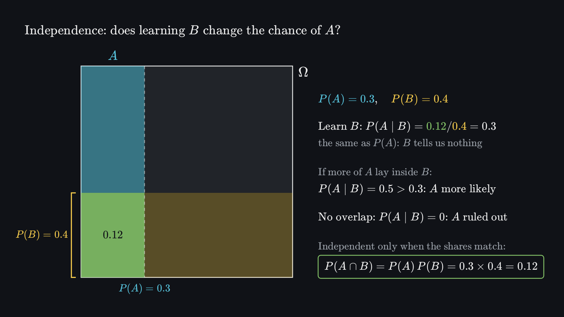
Before it plays Before playing, predict: if A and B did not overlap at all, would they be independent?
1.3.2Reversing a condition
Bayes’ rule rebuilds the reverse condition from the known one
Key formula Result (7)
Bayes’ rule
In words write P(H∩E) both ways with (4), equate, divide by P(E).
Needs P(E)>0; the denominator comes from (5).
Definition
Prior, likelihood, posterior
Prior P(H): before the evidence.
Likelihood P(E∣H): how readily H produces E.
Posterior P(H∣E): after the evidence.
Evidence favours H only if it is more likely under H than under the alternatives.
1.3.3Worked example
A positive test: count both routes to a positive result
D: uses EPO, P(D)=0.15. +: positive test, with P(+∣D)=0.90 and P(+∣Dc)=0.12.
Worked example
- Users who test positive: 0.90×0.15=0.135
- Non-users who test positive: 0.12×0.85=0.102
- All positives, by (5): 0.135+0.102=0.237
- By (7): P(D∣+)=0.135/0.237≈0.57
| + | − | Total | |
|---|---|---|---|
| Users | 135 | 15 | 150 |
| Non-users | 102 | 748 | 850 |
| Total | 237 | 763 | 1,000 |
Row of users: 135/150=0.90.
Column of positives: 135/237≈0.57.
0.90 starts with users; 0.57 starts with positive tests.
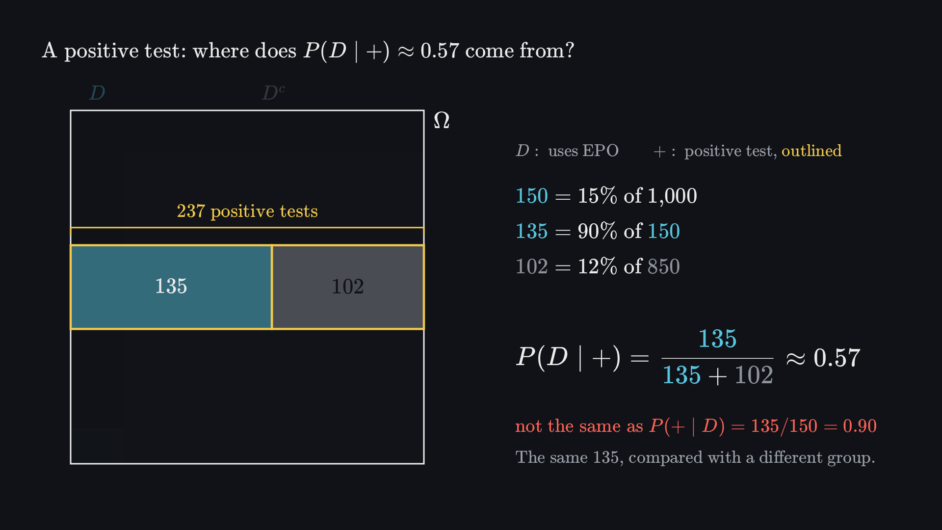
Before it plays Before playing, guess roughly what share of positive tests come from EPO users. The animation then traces every count in a hypothetical group of 1,000 cyclists.
1.3.4–5Evidence and assumptions
Rare evidence is not a small posterior: base rates and assumptions decide
Definition
Base rate
The prior share of a condition in the population. With only 1% users, the same test gives 0.01(0.90)+0.99(0.12)0.01(0.90)≈7%.
Worked example the Sally Clark case
An argument squared a single-death frequency of sudden infant death: (1/8,500)2=1/72,250,000.
Two separate errors
- Unsupported independence. Squaring needs P(S2∣S1)=P(S2); a shared family risk makes it larger.
- The prosecutor’s fallacy. A small P(E∣H) is not a small P(H∣E): rival explanations must be compared, with their priors.
Why economists care
The same logic governs screening, fraud detection and credit scoring: a signal’s meaning depends on how common each type is.
Review · How the ideas connect
One model, three moves: add, condition, reverse
Part 1 · Describe
Part 2 · Condition
Part 3 · Learn
Review · Summary sheet
What to take away: the terms and the seven formulas
Key terms
1 Describe
outcome ω: one possible result.
sample space Ω: the set of all outcomes the model considers.
event A⊆Ω: the outcomes that make a statement true.
disjoint A∩B=∅: no outcome in both.
The axioms of probability nonnegativity, P(Ω)=1, and disjoint events add.
2 Condition
conditional probability P(A∣B): the probability of A within the information event B.
partition disjoint groups Bi that together cover Ω.
3 Learn
Independence P(A∩B)=P(A)P(B): learning one event leaves the other’s probability unchanged.
Prior P(H): belief in a hypothesis before the evidence.
Likelihood P(E∣H): how readily H produces the evidence.
Posterior P(H∣E): belief after the evidence.
Base rate the prior share of a condition in the population tested.
Key formulas
1 Describe
2 Condition
3 Learn
Review · Back to the opening question
The cyclist: about 57%, not 90%
Result the opening question
0.90 is P(+∣D): it starts with users. We wanted the reverse, which starts with positive tests:
P(D∣+)=0.2370.135=7945≈0.57The test moved the probability from 15% to about 57%: strong evidence, far from certainty.
Remember
- Name the outcomes and the event before calculating.
- Every conditional names a group: divide by its size.
- Disjointness lets you add; independence lets you multiply.
Before next time
- Read notes 1.1–1.3 and the formula reference.
- Exercises 1.1.6, 1.2.5 and 1.3.6, with worked solutions.
- Watch the four animations not shown today.
Next · Lecture 2
Data, variables & moments. From events to measurements: random variables, distributions, expectation and variance.