Probability & Statistics · Lecture 3 of 5
Statistics
What can one sample tell us about a population, and how sure can we be?
1 Sampling→2 Intervals→3 Tests
- 1Probability theoryWhat can happen, and how does information change it?
- 2Data, variables & momentsHow do measurements vary?
- 3StatisticsWhat can one sample tell us about a population?
- 4Time seriesWhat changes when observations depend on their past?
- 5Causal inferenceWhich comparison identifies an effect?
Developed from Ian Crawford’s lecture material. Notes, slides and PDF: fatih.ai/probabilityandstatistics
Opening question
Smoking falls from 30% to 25% in both tables. Is the evidence the same?
100 people in a cessation programme, asked before and after; two constructed teaching tables with the same margins.
| smokes | not | |
|---|---|---|
| smokes | 20 | 10 |
| not | 5 | 65 |
| smokes | not | |
|---|---|---|
| smokes | 25 | 5 |
| not | 0 | 70 |
Your answer
Vote now. Part 2 answers it.
Why start here
Before-and-after data on the same people are everywhere in programme evaluation. Whether a change is real depends on how the data were collected, not only on the headline percentages.
Lecture 3 · The route
From one sample to a range for the truth and a verdict on a claim
Part 1
Samples and sampling distributions
What can one sample tell us about a population, and how much would another sample differ?
populationiidestimatorstandard errorCLT
Notes 3.1–3.3
Part 2
Confidence intervals
How precisely can one sample pin down a mean, a proportion or a difference, and what does “95% confidence” promise?
confidence intervalcoveragecritical valuepaired data
Notes 3.4–3.5
Part 3
Hypothesis tests
When is a sample result strong enough evidence against a claim, and what do α, the p-value and “fail to reject” actually say?
null hypothesisType I errorpowerp-valueduality
Notes 3.6–3.8
By the end of this lecture you can
- Distinguish a parameter, an estimator and an estimate, and say what the selection mechanism lets a sample tell us.
- Derive the standard error σ/n, and use the LLN and CLT to justify an approximately normal estimate.
- Construct and interpret 95% intervals for a mean, a proportion or a difference, matching the SE to the design.
- Carry out a two-sided z test and interpret α, power and the p-value correctly.
1
Part 1 of 3
Samples and sampling distributions
What can one sample tell us about a population, and how much would another sample differ?
Key terms
populationiidestimatorstandard errorCLTWhy it matters
Economists mostly work with samples: income surveys, polls and experiments. A sample average is informative only if the way units were selected targets the right population, and only as precise as its standard error.
In this part
- 3.1Who is sampled, and how
- 3.2Parameter, estimator and estimate
- 3.2Bias and the standard error
- ▶Animation: where the square root of n comes from
- 3.3The law of large numbers and the central limit theorem
3.1Target, design and iid
Say who is sampled and how before using any formula
Definition
Population and sample
The population is what we want to describe; the sample is what a stated selection mechanism delivers from a frame, the list units are drawn from.
- Who is missing from the frame?
- Who is selected, and who responds?
- Which steps are random?
Common mistake
More respondents do not remove nonresponse bias: a very large sample from the wrong group answers the wrong question very precisely.
Definition
iid
Independent and identically distributed: the draws are jointly independent and each has the same distribution.
Worked example ten examination scripts, one graded 90
Draw two without replacement. Before any draw, P(X2=90)=1/10, the same as X1. But
P(X2=90∣X1=90)=0=101.Identical, yet dependent. With replacement, the draws are iid.
3.2Parameter, estimator, estimate
A parameter is fixed, an estimator is a random rule, an estimate is one number
| Object | Random? | Example |
|---|---|---|
| Parameter θ | fixed, unknown | population mean μ |
| Estimator θ^ | random | Xˉ |
| Estimate | a number | xˉ=2.5 |
Definition
Sampling distribution
The distribution of an estimator across repeated samples, not the spread of the data within one sample.
Key formula Definition (1)
Sample mean and variance
In words divide by n−1: the n deviations obey one constraint.
Worked example six observations: 1, 2, 1, 3, 4, 4
xˉ=15/6=2.5; the squared deviations sum to 9.5, so
s2=9.5/5=1.9,s≈1.378.3.2Bias and standard error
Judge an estimator by its centre and its spread: bias and standard error
Definition
Bias
Bias(θ^)=E[θ^]−θ, averaged over repeated samples. Xˉ is unbiased: E[Xˉ]=μ needs only common means.
Key formula Result (2)
Standard error of the mean
In words estimated by s/n.
Needs independent draws with a common variance; dependence adds covariance terms.
Worked example one score against the mean of 20
Scores uniform on 0, …, 100: σ2=850, so one score has SD 850≈29.15. The mean of 20 independent scores has
SE=850/20=2029.15≈6.52.Common mistake
The SD describes individuals; the standard error describes the estimator across samples. For 1, 2, 1, 3, 4, 4: s≈1.378 but SE≈0.563.
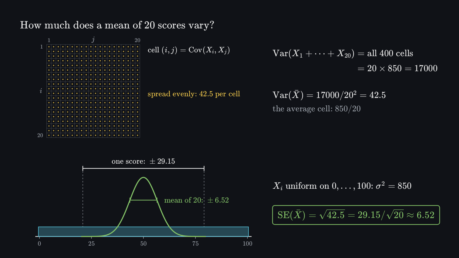
Before it plays Before playing, predict: one score has SD 29.15. Is the SD of a mean of 20 scores 29.15, 29.15/20 or 29.15/20?
3.3Large samples
Averages concentrate, and their errors become approximately normal
Result the law of large numbers
For iid data with finite mean and variance, Xˉn converges in probability to μ: P(∣Xˉn−μ∣>ε)→0.
Key formula Result (3)
Central limit theorem
In words for large n, Xˉn is approximately N(μ,σ2/n), and s may replace σ.
Needs iid data with 0<σ2<∞.
Worked example a U-shaped population
A Beta(21,21) variable has SD 0.3536. Means of 50 have SE (1/8)/50=0.05 and a bell-shaped histogram; at n=200 the SE halves to 0.025. The data stay U-shaped.
Common mistake
- The CLT is about means, not the data.
- There is no universal “n=30”.
- No sample size cures a biased selection.
An estimate is one draw from a sampling distribution: centred on its target if unbiased, with spread σ/n.
2
Part 2 of 3
Confidence intervals
How precisely can one sample pin down a mean, a proportion or a difference, and what does “95% confidence” promise?
Key terms
confidence intervalcoveragecritical valuepaired dataSo far an estimate is one draw from a sampling distribution; its standard error σ/n measures the spread, and the CLT makes it approximately normal.
Why it matters
Decisions need a range, not a point. A 39% approval rate means little without its 2.47-point margin, and a fall in smoking after a programme is convincing or not depending on how many people actually changed.
In this part
- 3.4A confidence interval and its coverage
- ▶Animation: what the 95% in a confidence interval describes
- 3.4One recipe, three designs
- 3.5A proportion is a mean of 0/1 data
- 3.5The opening question answered
3.4Building an interval
A confidence interval turns a statement about the estimate into a range for the target
Key formula Result (4)
Confidence interval for a mean
In words P(Xˉ−cSE≤μ≤Xˉ+cSE)=1−α: the random interval covers the fixed μ with probability 1−α.
Needs exact for normal data with known σ; approximate for large samples with s/n.
Definition
Coverage
The share of repeated samples whose interval contains the parameter. It belongs to the procedure, not to one computed interval.
| Confidence | 90% | 95% | 99% |
|---|---|---|---|
| c | 1.645 | 1.960 | 2.576 |
Result width
The width is 2cSE: more confidence widens it; four times the sample size halves it.
The algebra moves the randomness to the endpoints; μ stays fixed.
![Final frame: the sampling distribution of the mean, N(0, 1/5), with its central 95% between −0.877 and 0.877 shaded and its two 2.5% tails in red; dashed lines continue the band’s edges down the page, and a fixed dashed line marks μ = 0. Below, 40 simulated intervals x̄ ± 0.877: those whose mean lies inside the band cross the μ line (green); 3 whose mean lies outside miss it (red). Beside it: n = 5 from N(0, 1), X̄ ~ N(0, 1/5); 1.96/√5 ≈ 0.877, so P(|X̄ − μ| ≤ 0.877) = 0.95; each sample gives the interval x̄ ± 0.877; 1.00 ± 0.877 = [0.123, 1.877] misses 0; a miss happens exactly when x̄ lands outside the 95% band; this run: 37 of 40 contain 0; 95% describes the procedure over many samples, and one computed interval either contains μ or not.](media/coverage-end.png?v=3306c2f419)
Before it plays Before playing, predict: once one 95% interval has been computed, is there a 95% chance that it contains μ?
3.4Means in three designs
One recipe, three designs: the design decides the standard error
| Design | Example | Estimate | SE | 95% interval |
|---|---|---|---|---|
| One mean | n=100, xˉ=64, s2=8 | 64 | 0.283 | [63.446, 64.554] |
| Independent groups | anchoring prompt 10 vs 65 (43 and 46 students) | −13.6 | 7.5≈2.739 | [−18.968, −8.232] |
| Paired | 71 students, exam 1 minus exam 2 | −1.8 | 124.45/71≈1.324 | [−4.395, 0.795] |
Key formula Result (5)
Standard errors by design
In words independent groups: variances add. Paired: analyse the n differences, sD2=sX2+sY2−2sXY.
Common mistake
Treating paired scores as independent: 117/71+151/71 ignores the positive covariance and overstates the SE. And [−4.395,0.795] including 0 does not prove the means equal.
3.5Proportions
A proportion is a mean of 0/1 data, with its own standard error
Key formula Result (6)
Interval for a proportion (Wald)
In words Var(p^)=p(1−p)/n, estimated by plugging in p^.
Needs a large iid sample, away from 0 and 1.
Common mistake
At 0 successes in 10 the Wald interval is [0,0]. Clipping does not repair it; the Wilson interval, about [0,0.2775], does better.
Worked example an approval survey
n=1502, p^=0.39, treated as an iid unweighted sample:
SE=15020.39(0.61)≈0.01260.39±1.96(0.0126): from 36.53% to 41.47%, a margin of about 2.47 percentage points, not 2.47%.
3.5Paired proportions
Same fall from 30% to 25%, different uncertainty: the people who changed decide
Each person’s change Di is −1 (quit), 0 (no change) or +1 (start). The SE is sD/n, and only people who changed contribute to sD.
| smokes | not | |
|---|---|---|
| smokes | 20 | 10 |
| not | 5 | 65 |
| smokes | not | |
|---|---|---|
| smokes | 25 | 5 |
| not | 0 | 70 |
Worked example the two tables
Table A: sD2=14.75/99, SE ≈0.0386:
−0.05±1.96(0.0386)≈[−0.126, 0.026]Table B: sD2=4.75/99, SE ≈0.0219:
−0.05±1.96(0.0219)≈[−0.093, −0.007]B’s interval rests on only five changes, so an exact test is safer; and a before–after fall is not, by itself, the programme’s effect.
The interval is estimate ± critical value × SE, with the SE matched to the design: one sample, independent groups or pairs.
3
Part 3 of 3
Hypothesis tests
When is a sample result strong enough evidence against a claim, and what do α, the p-value and “fail to reject” actually say?
Key terms
null hypothesisType I errorpowerp-valuedualitySo far a 95% interval is the estimate ±1.96 standard errors, with the standard error matched to the design.
Why it matters
Economists test claims and act on them: an evenly split electorate, no anchoring effect, no change after a programme. Reading a p-value as the probability that a claim is true, or “not significant” as “no effect”, produces false findings.
In this part
- 3.6What a test controls
- 3.6One test from start to finish
- ▶Animation: what a p-value is an area of
- ▶Animation: what a stricter level costs in power
- 3.7Tests for means and proportions
- 3.8A confidence interval is the set of nulls not rejected
3.6Hypotheses and error rates
A test limits how often it rejects a true claim, not the chance that the claim is true
State H0:θ=θ0 against H1:θ=θ0 about a parameter, with the direction and level fixed in advance.
| H0 true | H0 false | |
|---|---|---|
| Reject | Type I error | correct: power |
| Do not reject | correct | Type II error |
Key formula Definition (7)
Level and power
In words power 1−β(θ) is the probability of rejecting at a given alternative.
Check
A 5% test rejects. Is there now a 5% chance that H0 is true?
Answer
No: α bounds P(reject∣H0), not P(H0∣reject). Reversing the condition needs Bayes’ rule (Lecture 1).
Many tests
Run 20 tests of true nulls at 5% and 1−0.9520≈0.64 is the chance of at least one false finding. Bonferroni uses α/m.
3.6The statistic and the p-value
Count the standard errors from the claim; the p-value is the tail beyond them
Key formula Definition (8)
Test statistic
In words the distance from the claim in null standard errors; reject at 5% if ∣Z∣>1.96.
Key formula Definition (9)
Two-sided p-value
In words the probability, if H0 were true, of a statistic at least as extreme as the one observed.
Worked example H0:μ=64.5
- xˉ=64, SE 8/100≈0.283.
- z=(64−64.5)/0.283≈−1.77.
- pval=2{1−Φ(1.77)}≈0.077.
- 0.077>0.05: fail to reject. Report 64, [63.45,64.55] and pval≈0.077.
Common mistake
“We failed to reject, so μ=64.5.” The data are just as compatible with 64.3.
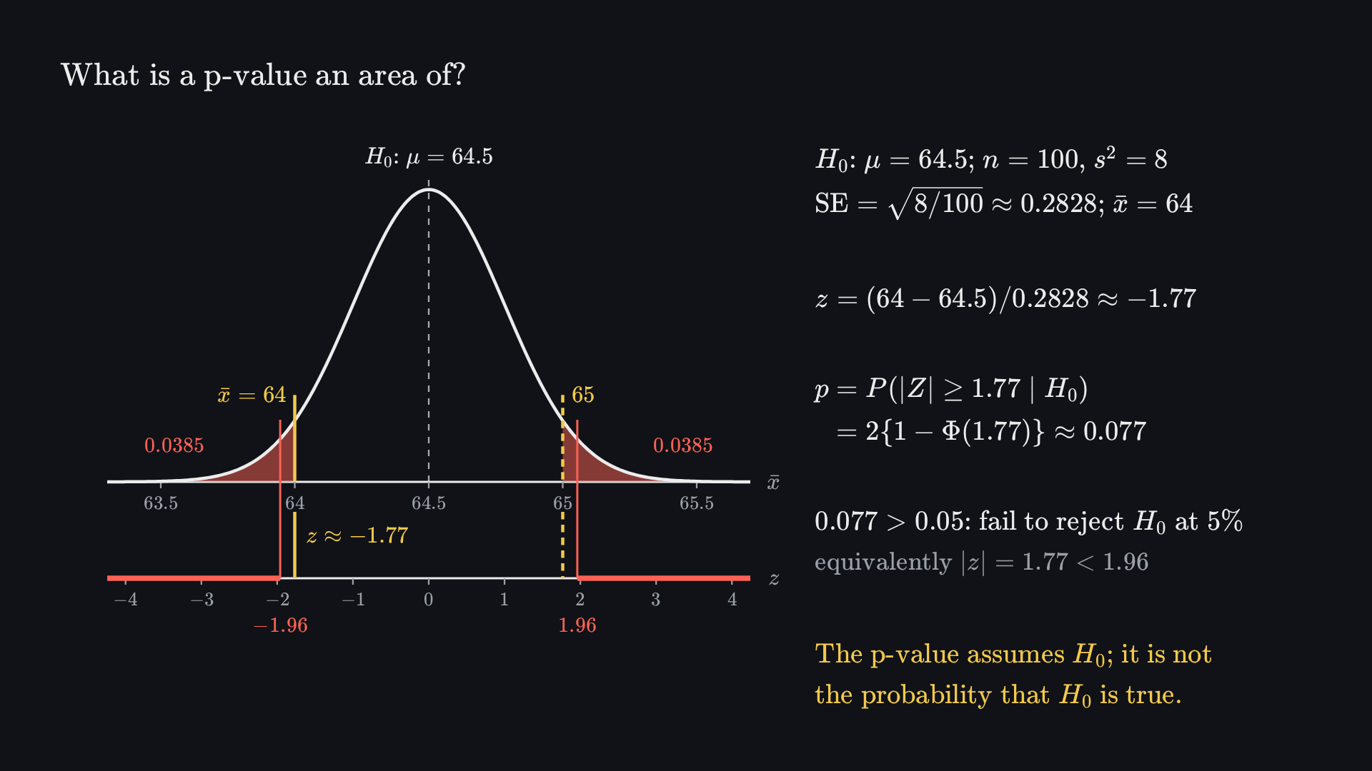
Before it plays Before playing, predict: the sample mean lies 1.77 standard errors below the claimed 64.5. Is that significant in a two-sided test at 5%?
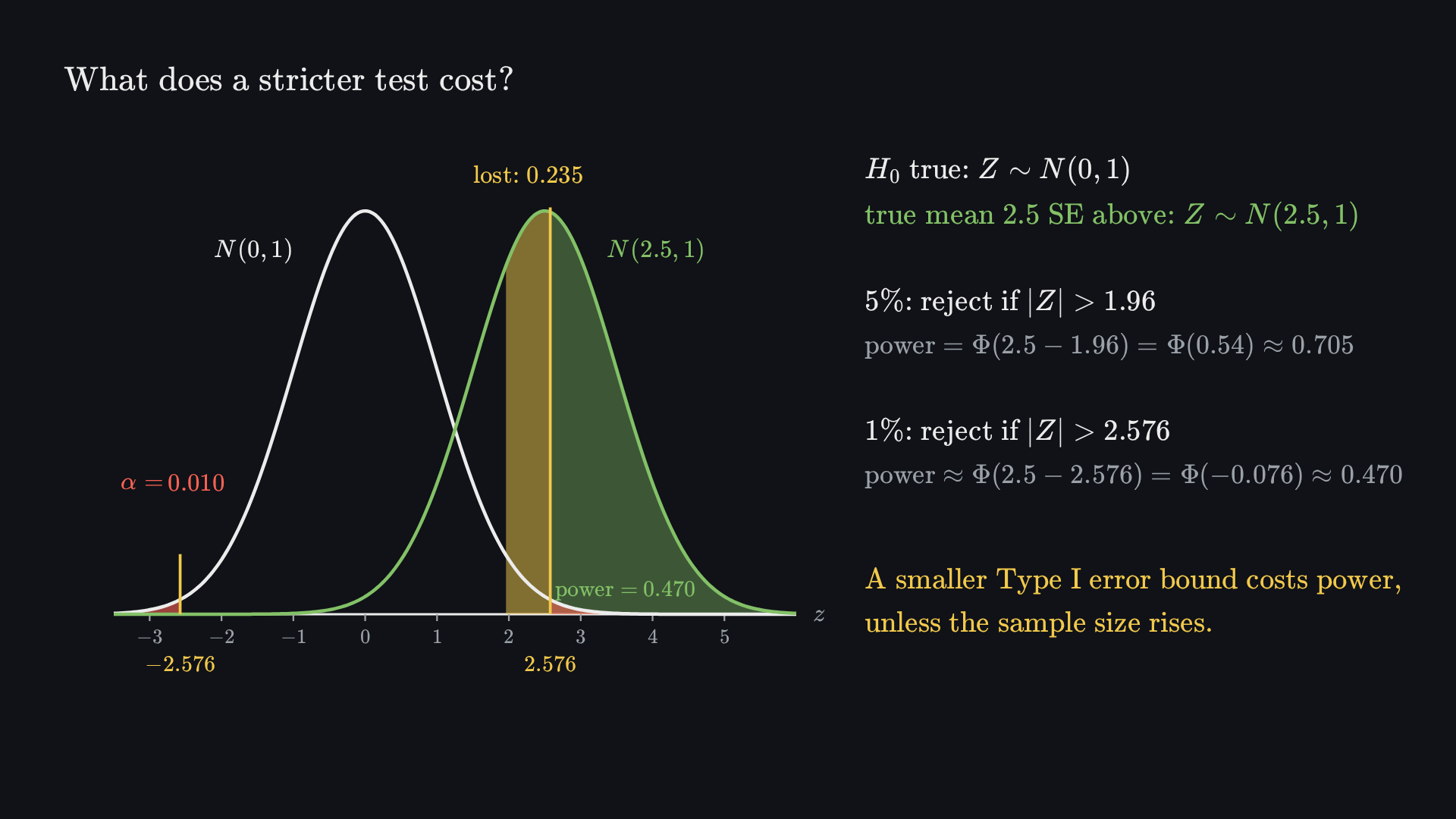
Before it plays Before playing, predict: if a two-sided test at 5% is made stricter, at 1%, what happens to its chance of detecting a real effect?
3.7Tests by design
The same designs as the intervals, with the standard error computed under the null
| Design | H0 | SE under H0 | z | pval | At 5% |
|---|---|---|---|---|---|
| One mean | μ=65 | s/n=0.283 | −3.54 | 0.0004 | reject |
| Independent means | no anchoring effect | 7.5 | −4.97 | <0.0001 | reject |
| Paired means | equal exam means | 124.45/71 | −1.36 | 0.17 | do not reject |
| One proportion | p=0.5 | p0(1−p0)/n | −8.53 | <0.0001 | reject |
| Two proportions | pX=pY | pooled π^≈0.390 | 3.58 | 0.0003 | reject |
| Paired proportions | no change (Table A) | sD/n | −1.30 | 0.20 | do not reject |
Common mistake
For proportions the null fixes the SE: use p0, not p^, for one proportion, and pool only when testing equality.
3.8Tests and intervals agree
An interval is every claim the matching test keeps
Key formula Result (10)
Inverting a test
In words a value is retained by the test exactly when it lies in the interval.
Needs the same data, SE e, reference distribution, tails and level.
Report the estimate and its interval, not just “significant”: significant is not important, and not rejecting is not equivalence.
Worked example xˉ=64, SE 0.283, interval [63.446,64.554]
μ0=64.2: z≈−0.71, pval≈0.48, retained.
μ0=65: z≈−3.54, pval≈0.0004, rejected.
Common mistake
For a proportion the score test (SE from p0) inverts to the Wilson interval, not the Wald interval: only a matching pair agrees.
A test counts null standard errors from the claim; the interval is every claim it would not reject.
Review · How the ideas connect
One chain: design, estimator, standard error, then interval and test
Part 1 · Sampling
Part 2 · Intervals
Part 3 · Tests
Review · Summary sheet
What to take away: the terms and the ten formulas
Key terms
1 Sampling
population the collection or distribution we want to make a statement about.
iid independent draws, each with the same distribution.
Estimator θ^=g(X1,…,Xn): a rule applied to the random sample.
Sampling distribution how an estimator varies across repeated samples.
Bias E[θ^]−θ: the average error over repeated samples.
standard error the SD of an estimator’s sampling distribution.
2 Intervals
Coverage the share of repeated samples whose interval contains the parameter.
Critical value c=z1−α/2: 1.645, 1.960, 2.576 for 90, 95, 99%.
3 Tests
Type I error rejecting a true null hypothesis.
Key formulas
1 Sampling
2 Intervals
3 Tests
Review · Back to the opening question
Same 5-point fall; only Table B’s interval excludes zero
Result the opening question
The margins cannot decide it: the standard error comes from the people who changed. Table A, 15 changes: [−0.126,0.026]. Table B, 5 changes: [−0.093,−0.007].
Remember
- An estimate is one draw; its SE says how far another would land.
- 95% describes the procedure, not one computed interval.
- A p-value is computed assuming H0; it is not the probability that H0 is true.
Before next time
- Notes 3.1–3.8 with the worked solutions.
- The sampling, coverage, tails and duality figures in the notes.
- Rework the six tests in the table for yourself.
Next · Lecture 4
Time series. When observations depend on their past, they are not iid: what changes for models, forecasts and standard errors?