Probability & Statistics · Lecture 5 of 5
Causal inference
Which comparison answers the question “what if we intervene?”
1 Effects and selection→2 Designs→3 Adjustment
- 1Probability theoryWhat can happen, and how does information change it?
- 2Data, variables & momentsHow do measurements vary?
- 3StatisticsWhat can one sample tell us about a population?
- 4Time seriesWhat changes when observations depend on their past?
- 5Causal inferenceWhich comparison identifies an effect?
Developed from Ian Crawford’s lecture material. Notes, slides and PDF: fatih.ai/probabilityandstatistics
Opening question
The treated score 16.67 points lower. Did the treatment hurt them?
Seven people, outcomes in invented points. People 1, 3 and 4 were treated.
| Person | 1 | 2 | 3 | 4 | 5 | 6 | 7 | |
|---|---|---|---|---|---|---|---|---|
| Treated? | yes | no | yes | yes | no | no | no | |
| Outcome | 30 | 30 | 46 | 54 | 60 | 70 | 80 | treated mean 43.33, others 60 |
Your answerVote now. Part 1 answers it.
Why start here
Programme evaluations, university premiums and pay gaps all start from a comparison like this one. The question is what else differs between the groups.
Lecture 5 · The route
Define the effect, then find a comparison that identifies it
Part 1
The effect we want and the gap we see
What is a causal effect, and why does a difference in group averages not measure it?
potential outcomesATEATTselection bias
Notes 5.1–5.2
Part 2
Designs that remove selection
How can the way treatment is assigned make selection bias zero, and for whom is the answer then valid?
random assignmentITTcompliersLATEexternal validity
Notes 5.3, 5.4, 5.7
Part 3
Adjusting for covariates
Without randomisation, when does comparing like with like recover the effect, and when does “controlling for” make things worse?
CIAoverlaptarget weightsbad control
Notes 5.5–5.6
By the end of this lecture you can
- Define potential outcomes, ATE and ATT, and explain why one potential outcome per person is always missing.
- Derive Δ=ATT+B and argue the likely sign of selection bias in an economic comparison.
- Explain what random assignment identifies, and compute ITT and the Wald ratio for compliers.
- Judge an adjusted comparison: CIA, overlap, the right weights, and why occupation is a bad control for pay.
1
Part 1 of 3
The effect we want and the gap we see
What is a causal effect, and why does a difference in group averages not measure it?
Key terms
potential outcomesATEATTselection biasWhy it matters
People choose programmes, universities and jobs partly on their prospects, so participants differ from non-participants before any treatment. A naive comparison could close a helpful programme, or credit a university with earnings its students would have had anyway.
In this part
- 5.1Potential outcomes: one person, two outcomes, one observed
- 5.1ATE and ATT: whose effect?
- 5.2Every observed gap is ATT plus selection bias
- ▶Animation: how selection bias can hide a positive effect
- 5.2Selection can push a comparison either way
5.1Two worlds for one person
Each person has two potential outcomes; we only ever see one
Definition
Potential outcomes
For unit i and treatment Di∈{0,1}: Yi(1) is the outcome under treatment, Yi(0) without it. The individual effect is τi=Yi(1)−Yi(0). The outcome not realised is the counterfactual.
Key formula Identity (1)
The observed outcome
In words we observe Yi(1) if treated and Yi(0) if not, never both.
Needs a well-defined treatment, and no effect of one person’s treatment on another’s outcome.
One person, two possible outcomes, one observation
So τi is never observed for anyone: causal inference is a missing-data problem.
5.1Average effects
ATE and ATT average the same effects over different people
Key formula Definition (2)
Average treatment effects
In words the average effect over everyone, and over the treated. Both terms of an effect average over the same people.
ATE and ATT differ when effects vary and the treated are not typical: ATE=P(D=1)ATT+P(D=0)ATU.
| Person | D | Y(0) | Y(1) | τ |
|---|---|---|---|---|
| 1 | 1 | 20 | 30 | 10 |
| 2 | 0 | 30 | 32 | 2 |
| 3 | 1 | 40 | 46 | 6 |
| 4 | 1 | 50 | 54 | 4 |
| 5 | 0 | 60 | 64 | 4 |
| 6 | 0 | 70 | 80 | 10 |
| 7 | 0 | 80 | 78 | −2 |
ATE=34/7≈4.86; ATT=(10+6+4)/3≈6.67.
ATT subtracts the treated people’s own no-treatment outcomes, not the control group’s observed mean.
5.2An identity, not an assumption
Every observed gap is the effect plus selection bias
Key formula Identity (3)
Observed difference = effect + selection
In words add and subtract E[Y(0)∣D=1], the treated group’s unseen no-treatment mean.
Definition
Selection bias
B=E[Y(0)∣D=1]−E[Y(0)∣D=0]: how the treated would have fared untreated, compared with the untreated.
Worked example the toy population
The treated would have averaged 110/3 untreated; the controls average 60.
BΔ=110/3−60=−70/3≈−23.33=20/3−70/3=−50/3≈−16.67Common mistake
Selection bias is not sampling bias. It arises even when the whole population is observed.
Identification is whatever justifies learning the unseen E[Y(0)∣D=1].
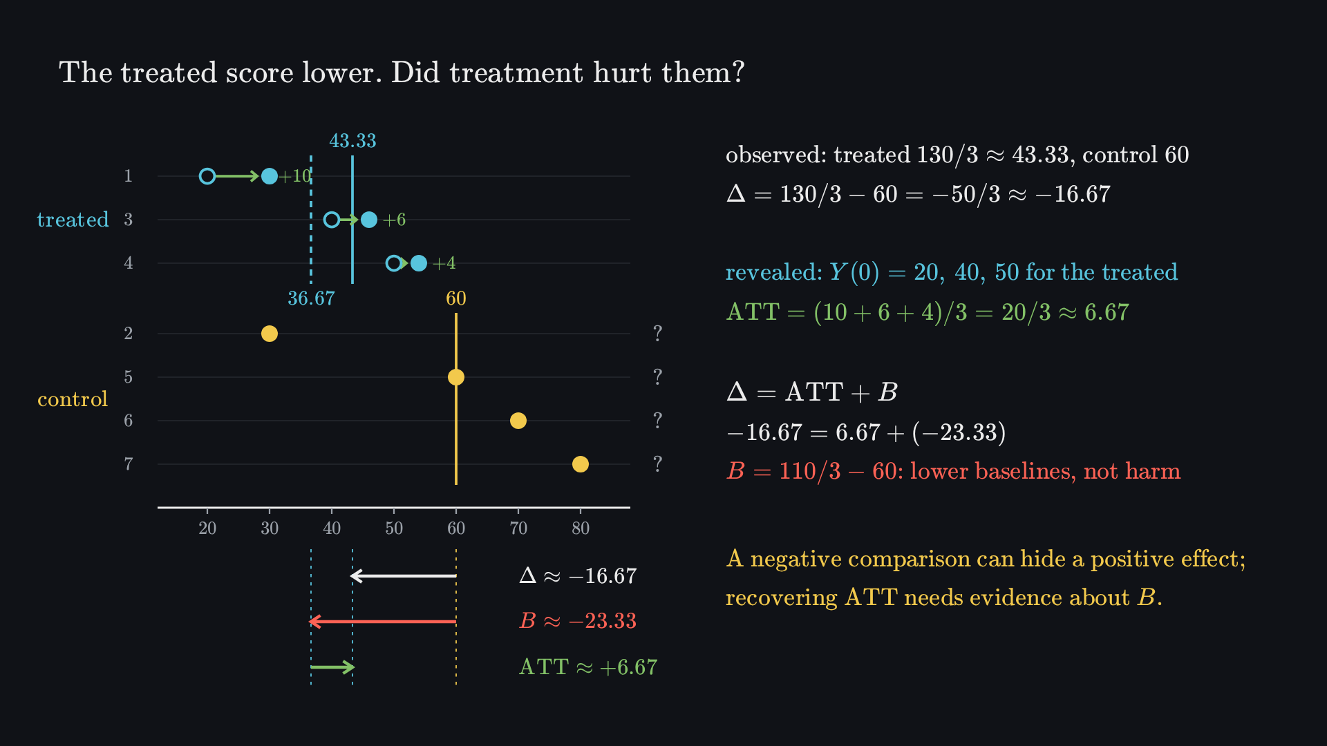
Before it plays Before playing, predict: the treated group scores 16.67 points below the controls. Does that mean treatment hurt them?
5.2Reading the sign of B
Selection can push a comparison either way
Worked example a university premium (illustration)
Graduates of university O earn £4,000 more than those of X: Δ=ATT+B. If O’s students would have earned more even at X, then B>0 and ATT<£4,000; B=£3,000 would leave £1,000.
Worked example a training programme (illustration)
Participants earn £8.80 a week less: Δ=−£8.80. If participant selection contributes −£12, then
ATT=−8.80−(−12)=+£3.20 a week.Why economists care
Closing a programme or justifying higher fees needs ATT, not Δ. Economists expect selection wherever people choose treatment on their prospects.
Check
Δ=12. Decompose it with ATT=5, and with ATT=15.
Answer
B=7 and B=−3. Both satisfy the identity; the data alone cannot choose.
2
Part 2 of 3
Designs that remove selection
How can the way treatment is assigned make selection bias zero, and for whom is the answer then valid?
Key terms
random assignmentITTcompliersLATEexternal validitySo far Δ=ATT+B always holds, and the data alone cannot say how large B is.
Why it matters
Randomised trials, offers and eligibility rules are the economist’s main evaluation tools. But people decline offers, effects spill over at scale and studies are short; each changes what is identified, and whether it carries over to a national policy.
In this part
- 5.3Random assignment: B = 0 on average
- 5.3, 5.7Compare by the offer: ITT, then LATE for compliers
- ▶Animation: the Wald ratio recovers the effect for compliers
- 5.4A credible trial need not transport
- 5.4Natural experiments and a threshold rule
5.3Random assignment
Random assignment sets selection bias to zero on average, not in every draw
Key formula Assumption (4)
Random assignment
In words assignment is independent of the pair of potential outcomes; then B=0 and Δ=ATT=ATE.
Needs the design assigns treatment with the same positive probability to every unit.
Common mistake
It does not make the observed Y independent of D: a treatment effect is exactly how assignment changes Y.
All 35 ways to treat three of the seven people:
Unbiased over allocations; one draw can still be far off. Inference (Lecture 3) measures that chance variation.
5.3, 5.7Offers and take-up
People refuse offers: compare by the offer, then rescale for compliers
Key formula Definition (5)
Intention to treat
In words Z is the randomised offer, D the treatment received. ITT is the effect of offering, take-up included.
| never-taker (0,0) | complier (0,1) |
| always-taker (1,1) | defier (1,0): ruled out |
Common mistake
Comparing takers with non-takers: take-up selects on motivation, so it forfeits the randomisation.
Key formula Result (6)
The Wald ratio: LATE
In words the offer’s effect on outcomes over its effect on take-up: the average effect for compliers.
Needs a random offer that affects Y only through D (exclusion), changes take-up, and creates no defiers.
LATE is local: a different offer moves different people, and its compliers may gain more or less than everyone else.
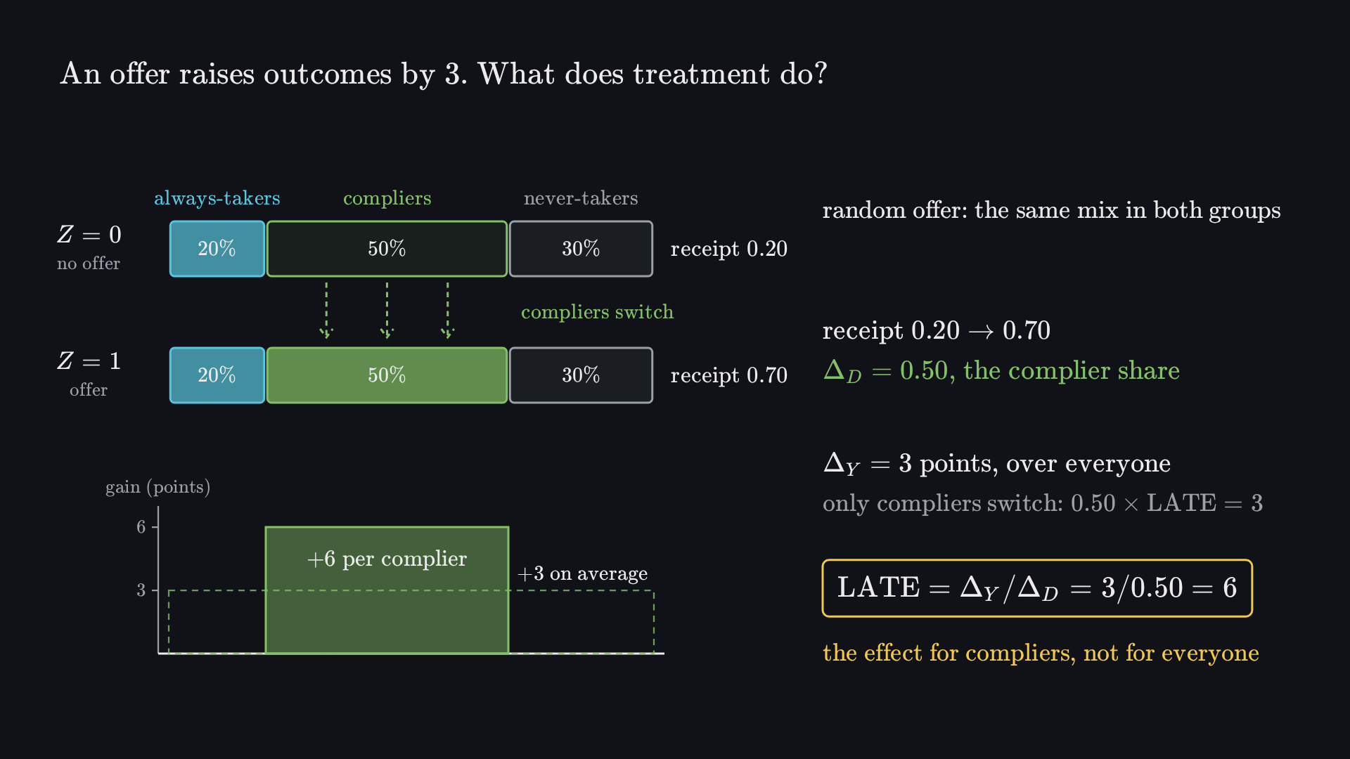
Before it plays Before playing, predict: a random offer raises average outcomes by 3 points and moves receipt from 20% to 70%. How large is the treatment’s effect for those who switch?
5.4Internal and external validity
A credible trial need not transport to another setting
Definition
Internal validity
Does the study credibly identify its stated effect for the units and treatment actually studied? Check assignment, take-up, measurement, missing outcomes, interference.
Definition
External validity
Does the result transport to another population, setting, implementation or time horizon? Check people, institutions, scale, follow-up.
Why a good trial may not carry over
- Spillovers. If treating one person affects others, outcomes are Yi(di,d−i): a pilot and a national policy are different interventions.
- Surrogates. An exam score next term is not earnings in ten years.
- Being observed. Hawthorne and placebo effects: define the comparison; blind where possible.
Good random assignment supports internal validity without establishing external validity.
5.4Natural experiments
A natural experiment is an argument, not a label
Definition
Natural and quasi-experiments
Variation from outside the researcher’s control that resembles random allocation in the relevant respect. Name the source of variation, the comparison, the competing pathways and the local target.
Common mistake
“The weather was random.” A storm’s exposure varies with location and housing, and it can hit income directly, not only through moving house.
Worked example a class-size threshold rule
With classes capped at 40, enrolment n predicts class size
q(n)=⌈n/40⌉n| n=40 | 40 | n=80 | 40 |
| n=41 | 20.5 | n=81 | 27 |
One more pupil drops the predicted size by 13. Compare schools just either side, if nothing else jumps at 40 and schools cannot sort.
3
Part 3 of 3
Adjusting for covariates
Without randomisation, when does comparing like with like recover the effect, and when does “controlling for” make things worse?
Key terms
CIAoverlaptarget weightsbad controlSo far randomisation sets B=0 by design; a random offer identifies ITT and, under conditions, LATE for compliers.
Why it matters
Most economic data are observational, and adding controls is routine. Whether the gender pay gap “disappears within occupations” turns on exactly this question.
In this part
- 5.5CIA: as good as random within covariate cells
- 5.5Same cell effects, different targets
- 5.5No comparison without overlap
- 5.6Composition and the pay gap
- 5.6Control for confounders, not for outcomes of treatment
- ▶Animation: equal pay within a profession can hide a negative effect
5.5Selection on observables
Conditional independence: within covariate cells, assignment is as good as random
Key formula Assumption (7)
Conditional independence (CIA)
In words within each group of pre-treatment covariates X, assignment is independent of the potential outcomes.
Needs an argument about how treatment was assigned. Then τ(x)=m1(x)−m0(x), the within-cell difference of observed means.
What CIA does not say
- CIA does not say potential outcomes are constant within a cell.
- No number of controls makes it true, and balance on observed variables does not test it.
Worked example military service and earnings
Compare applicants who enlisted with applicants who did not, holding recorded screening characteristics fixed. Threat: persistence or reliable attendance may drive both enlistment and later earnings.
5.5Averaging cell effects
The same cell effects give different answers for different targets
Key formula Result (8)
Target weights
In words ATE weights cells by the population; ATT by the treated.
Check
Cell effects 3 and 9; population shares 0.7 and 0.3; treated shares 0.2 and 0.8. ATE and ATT?
Answer
ATE=4.8, ATT=7.8.
Worked example two cells, half the population each
Treatment probability 0.2 in cell X=0, 0.8 in cell X=1.
| Cell | Population | Treated | τ(x) |
|---|---|---|---|
| X=0 | 0.5 | 0.2 | 2 |
| X=1 | 0.5 | 0.8 | 6 |
The raw gap, 23.2−12=11.2, adds baseline selection of 6.
5.5Overlap and sparse cells
No comparison without overlap, and fine cells empty fast
Key formula Assumption (9)
Overlap (common support)
In words at every covariate value in the target, some units are treated and some are not.
Needs for ATT, untreated comparisons wherever treated people are. It can be checked in the data.
Common mistake
If everyone with X=1 is treated, τ(1) is not identified: a fitted model fills the cell only by extrapolation, and trimming changes the estimand.
Worked example 100 points spread evenly over k variables
Expected count in a cell of side 0.2 of each range:
| k | 1 | 2 | 3 | 4 | 5 |
|---|---|---|---|---|---|
| count | 20 | 4 | 0.8 | 0.16 | 0.032 |
To expect 5 points with k=5, each side must be (0.05)1/5≈0.55 of its range.
5.6Composition
Composition alone can make the overall gap exceed every within-group gap
Published statistic ONS 2021, provisional, UK medians
Median hourly-pay gaps: 7.9% full-time, −2.7% part-time, 15.4% overall. They compare pay across jobs, not people in the same job.
Common mistake
Medians cannot be averaged across groups: the law of iterated expectations is about means.
Worked example a hypothetical mean model
| Men | Women | Men’s share | Women’s share | |
|---|---|---|---|---|
| Full-time | 14.81 | 13.64 | 0.85 | 0.58 |
| Part-time | 9.07 | 9.31 | 0.15 | 0.42 |
Means 13.949 and 11.8214: a gap of 15.25%, above both within-stratum gaps (7.90% and −2.65%), because more women work in the lower-paid stratum.
5.6Bad controls
Control for confounders, not for outcomes of the treatment
A confounder: X causes both D and Y. Conditioning on it can help.
A pre-treatment common cause
A bad control: W is caused by D. Holding it fixed changes who is compared.
Selection through an outcome
Key formula Identity (10)
Comparing within an occupation
In words the gap among professionals = an effect for those who would be professional if treated + a difference in who becomes professional.
Needs D independent of all potential earnings and occupations jointly.
Definition
Bad control
A variable caused by the treatment, such as occupation for pay. Conditioning on it can hide part of the effect or create selection.
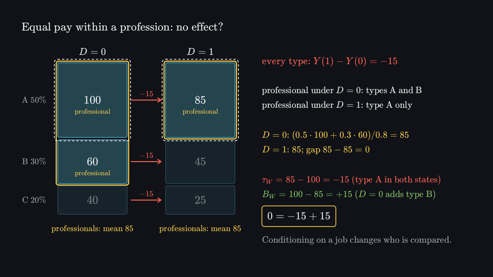
Before it plays Before playing, predict: among professionals, both groups earn 85. Does that show the treatment has no effect on earnings?
Review · How the ideas connect
One identity, three ways to deal with selection
Part 1 · Effects
Part 2 · Designs that set B = 0
Part 3 · Adjustment
the selection-bias identity
Review · Summary sheet
What to take away: the terms and the ten formulas
Key terms
1 Effects and selection
Potential outcomes Yi(1), Yi(0): one unit’s outcomes with and without treatment; one is always missing.
ATE the average effect over everyone.
ATT the average effect among the treated.
Selection bias the groups’ difference in no-treatment outcomes.
2 Designs
Random assignment assignment independent of the potential outcomes.
complier takes the treatment if and only if offered.
LATE the average effect for the compliers of one instrument.
Internal and external validity credible for the units studied; carries over to other settings.
3 Adjustment
CIA within covariate cells, assignment independent of potential outcomes.
Overlap treated and untreated units at every target covariate value.
Bad control a variable the treatment changes; conditioning on it alters who is compared.
Key formulas
1 Effects and selection
2 Designs
3 Adjustment
Review · Before you report a causal estimate
Name the target, defend the assumption, then measure the uncertainty
Before you report a causal estimate
- The intervention, population, outcome and time horizon.
- How treatment was assigned.
- The identifying condition: randomisation, exclusion, or CIA with overlap.
- Only then, inference suited to the design. A confidence interval does not cover a failed assumption.
Result the opening question
From the data alone: cannot tell. In the model, every treated person gained (ATT ≈+6.67); their lower baselines (B≈−23.33) produced the gap.
The course in one line
Probability defines uncertainty; distributions and moments describe measurements; statistics studies sampling variation; time series accounts for dependence over time; causal inference decides which comparison answers an intervention question.
Practise
Notes 5.1–5.7 with worked solutions; the five interactive figures (potential outcomes, selection, the 35 allocations, target weights, pay mixtures).