Probability & Statistics · Lecture 2 of 5
Data, variables & moments
How do measurements vary, and how do we summarise and relate them?
1 Describe→2 Summarise→3 Relate
- 1Probability theoryWhat can happen, and how does information change it?
- 2Data, variables & momentsHow do measurements vary?
- 3StatisticsWhat can one sample tell us about a population?
- 4Time seriesWhat changes when observations depend on their past?
- 5Causal inferenceWhich comparison identifies an effect?
Developed from Ian Crawford’s lecture material. Notes, slides and PDF: fatih.ai/probabilityandstatistics
Opening question
Ten exam scripts: what mark should you expect from one drawn at random?
Puzzle 1
(a) What mark should you expect? Does any script have it?
Puzzle 2
(b) Women’s four scripts average 72.5, men’s six average 58.33. Is the class mean halfway, 65.42?
Why start here
A national average wage built from group averages raises the same question: which weights, and why?
Lecture 2 · The route
Describe the variation, summarise it, then relate it to another variable
Part 1
Describe: from records to distributions
How likely is each value, each interval, each threshold?
random variablePMFdensityCDFquantile
Notes 2.1–2.4
Part 2
Summarise: centre, spread and the standard normal
Where is a distribution centred, how spread out is it, and how far from typical is a given value?
expectationvariancestandard deviationstandardiseΦ
Notes 2.5–2.7
Part 3
Relate: joint, conditional and association
What does knowing one variable tell us about another?
jointmarginalconditional meancovariancecorrelation
Notes 2.8–2.10
By the end of this lecture you can
- Classify a variable by type, support and structure, and read probabilities and quantiles from a PMF, density or CDF.
- Compute and interpret a mean, variance and standard deviation, using linearity and the change-of-units rules.
- Standardise a normal variable to find probabilities, quantiles and central intervals from one table.
- Derive marginal and conditional distributions and means from a joint table, and tell independence from zero correlation.
1
Part 1 of 3
Describe: from records to distributions
How likely is each value, each interval, each threshold?
Key terms
random variablePMFdensityCDFquantileWhy it matters
Economic data mix codes, counts and amounts, recorded as cross-sections, time series and panels; the type decides which calculations mean anything. A distribution then answers questions such as what share of incomes lies at or below £x.
In this part
- 2.1Measurement, support and data structure
- 2.2A PMF and the binomial
- ▶Animation: why a density can exceed 1 while probability is area
- 2.3Densities: probability is area
- 2.4The CDF, intervals and quantiles
2.1What is being measured
Know what a number measures before calculating with it
Definition
Random variable
X:Ω→R gives each outcome a number. Its support is the set of values the model permits.
Common mistake
Health coded poor 0, fair 1, good 2 is ordered only: “2 is twice as healthy as 1” has no meaning.
| Type | Meaning | Example |
|---|---|---|
| Nominal | labels only | employed 1, unemployed 0 |
| Ordinal | order, not distance | poor, fair, good |
| Discrete | countable quantities | people in a household |
| Continuous | a continuum, modelled | height, a lifetime |
Structure: a cross-section Xi, a time series Xt, a panel Xit. GDP for 20 countries over 5 years with two records missing is an unbalanced panel of 98 records: rows, not independent evidence.
The mean of a 0/1 employment indicator is the employment rate; the mean of eye-colour codes is meaningless.
2.2Masses on values
A probability mass function puts probability on values; a binomial counts every sequence
Definition
Probability mass function (PMF)
pX(x)=P(X=x), with pX(x)≥0 and ∑xpX(x)=1.
Worked example ten exam scripts, one drawn at random
Marks 30, 30, 30, 60, 60, 80, 80, 80, 90, 100:
| x | 30 | 60 | 80 | 90 | 100 |
| pX(x) | 0.3 | 0.2 | 0.3 | 0.1 | 0.1 |
P(X≥80)=0.5; P(X=70)=0.
Key formula Result (1)
Binomial distribution
In words (kN) sequences with k successes, each with probability pk(1−p)N−k.
Needs N independent trials with a common p=P(success).
Two heads in three fair tosses: HHT, HTH, THH, so 3/8, not 1/8. Five in ten: 252/1024≈0.246.
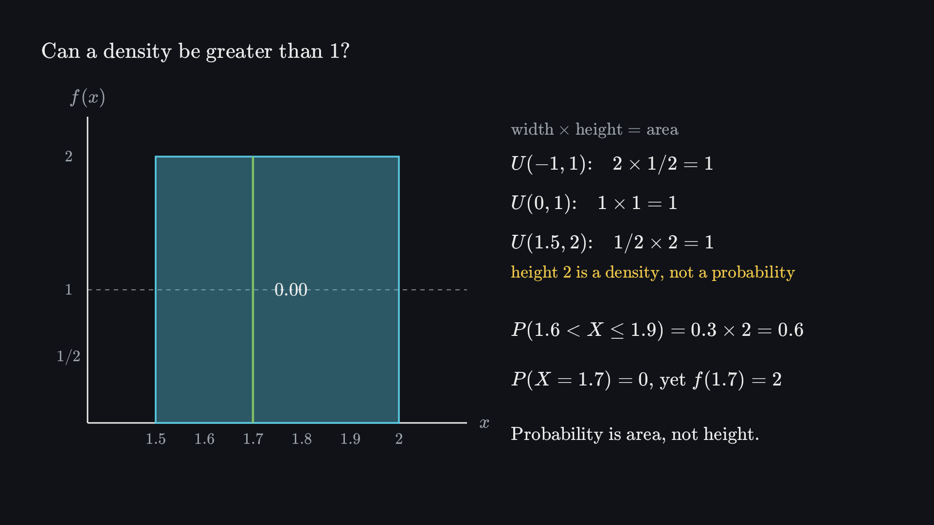
Before it plays Before playing, predict: can a density be greater than 1? And what is the probability of one exact value?
2.3Area under a density
For a continuous variable, probability is area under a density
Key formula Definition (2)
Probability from a density
In words the area under the curve between a and b; fX≥0 with total area 1.
Needs X has a density; then P(X=x)=0, so the endpoints do not matter.
Common mistake
A density of 2 is not a probability of 2: it is probability per unit. Clip intervals to the support: for U(−1,1), P(−2<X≤0.5)=1.5×21=0.75, not 1.25.
Shift location or change spread
Same spread
Same centre
A density family: N(μ,σ2) shifts with μ and widens with σ; the area stays 1.
2.4Accumulating probability
The CDF accumulates probability: subtract for intervals, read backwards for quantiles
Key formula Definition (3)
Cumulative distribution function
In words the probability up to a threshold, for every real x; a quantile reverses it: QX(p) is the lowest x with FX(x)≥p.
Common mistake
For the marks, P(30<X≤80)=0.8−0.3=0.5 but P(30≤X≤80)=0.8: the endpoint includes three scripts.
A jump adds the probability at its mark
The marks’ staircase: 0.3, 0.5, 0.8, 0.9, 1. Median QX(0.5)=60; the usual sample median, 70, is a different convention.
A PMF or density spreads probability 1; the CDF accumulates it, so intervals are differences of F and quantiles are F read backwards.
2
Part 2 of 3
Summarise: centre, spread and the standard normal
Where is a distribution centred, how spread out is it, and how far from typical is a given value?
Key terms
expectationvariancestandard deviationstandardiseΦSo far a distribution puts probability on values or areas; the CDF accumulates it and quantiles read it backwards.
Why it matters
Means and standard deviations are the first summary of wages, prices and returns. An expected payoff is not the likely payoff, and the standard normal scale is the yardstick for every interval and test in Lecture 3.
In this part
- 2.5The mean is a balance point
- 2.5Linear operations pass through expectations
- ▶Animation: why the variance squares deviations
- 2.6Variance and standard deviation
- ▶Animation: standardising keeps the event’s area
- 2.7Standardise, look up Φ, translate back
2.5The probability-weighted balance
The mean is a probability-weighted balance point, not a prediction
Key formula Definition (4)
Expected value
In words each value weighted by its probability; also called the mean.
Needs E[∣X∣]<∞.
Worked example the ten scripts
E[X]=30(0.3)+60(0.2)+80(0.3)+90(0.1)+100(0.1)=64No script has mark 64, and the most likely marks are 30 and 80.
The mean need not be a supported value
Why economists care
A payoff of 0 with probability 0.9 or 100 with probability 0.1 has mean 10 but mode 0. The expectation of a 0/1 indicator is a proportion.
2.5Transformations
Linear operations pass through expectations; nonlinear ones do not
Result linearity
E[a+bX]=a+bE[X],E[X+Y]=E[X]+E[Y]No independence needed. But E[XY]=E[X]E[Y] only under independence.
For the marks: E[5+0.8X]=5+0.8(64)=56.2.
Result Jensen’s inequality
For convex g, E[g(X)]≥g(E[X]); for concave g the reverse. For the marks: E[X2]=4720 but (E[X])2=4096.
Common mistake
The mean of log wages is not the log of the mean wage, and averaging ratios is not the ratio of averages: E[X/Y]=3/4 while E[X]/E[Y]=2/3 in the notes’ two-point example.
Changing units is safe; logs, squares and ratios are not. The gap 4720−4096 is the variance.
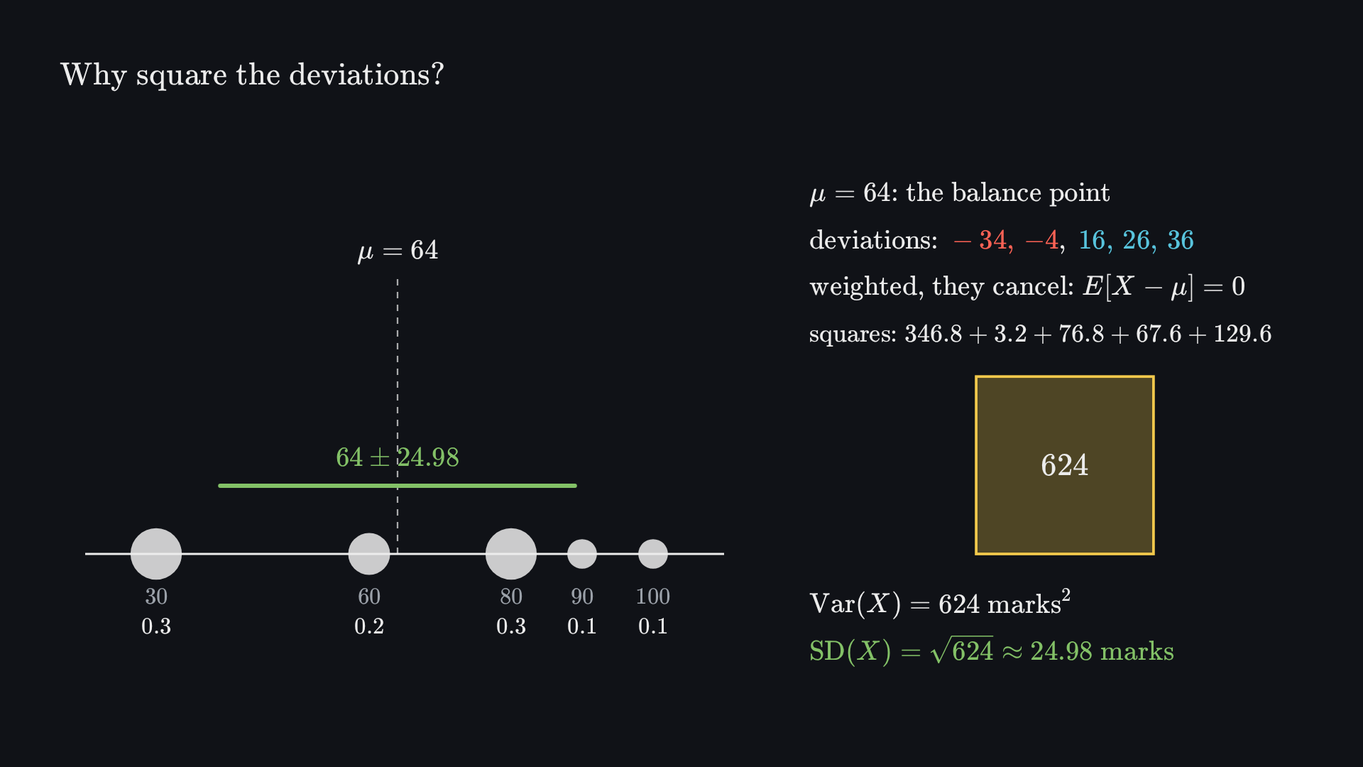
Before it plays Before playing, predict: what is the probability-weighted average of the deviations from the mean, 64? Why can it not measure spread?
2.6Spread
Variance averages squared deviations; the standard deviation returns to the original units
Key formula Definition (5)
Variance
In words the average squared distance from the mean; the standard deviation is its square root.
Result changing units
Var(a+bX)=b2Var(X),SD(a+bX)=∣b∣SD(X)Worked example the ten scripts
Var(X)=4720−4096=624 marks², so SD=624≈24.98 marks. For 10−2X: mean −118, SD ≈49.96.
Definition
A 0/1 variable
Mean p, variance p(1−p): the mean fixes the spread, at most 41. An average of N independent indicators has variance p(1−p)/N.
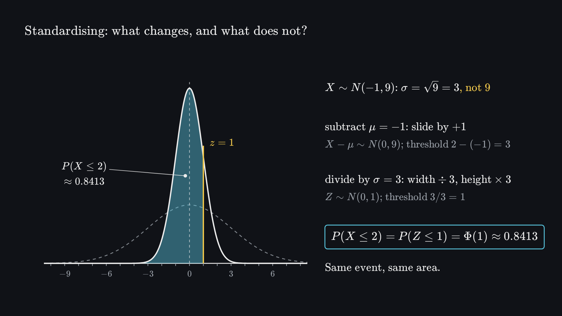
Before it plays Before playing, predict: to standardise X∼N(−1,9), do we divide by 9 or by 3? And does the shaded area change?
2.7One table for every normal
One table serves every normal: standardise, look up Φ, translate back
Key formula Result (6)
Normal probabilities and quantiles
In words Φ is the standard normal CDF; zp its quantile. Divide by σ, never σ2.
Needs X∼N(μ,σ2) with σ>0.
| z | −1 | 0 | 1 | 1.96 | 2 |
| Φ(z) | 0.1587 | 0.5 | 0.8413 | 0.9750 | 0.9772 |
Worked example a right tail
X∼N(0.2,1.5), so σ=1.5:
zP(X≥1.6)=(1.6−0.2)/1.5≈1.143=1−Φ(1.143)≈0.1265Common mistake
A central 95% interval leaves 2.5% in each tail, so it uses ±1.96, the 97.5th percentile, not the 95th (1.645). For N(−1,9): −1±3(1.96)=[−6.88,4.88].
The mean is the balance point, the variance the average squared distance; (x−μ)/σ puts any normal on one table.
3
Part 3 of 3
Relate: joint, conditional and association
What does knowing one variable tell us about another?
Key terms
jointmarginalconditional meancovariancecorrelationSo far the mean and variance summarise one variable; for a normal model (x−μ)/σ puts any question on one table.
Why it matters
Most economic questions compare groups or relate two measurements, such as earnings by gender or age. Conditional means are what regression estimates; covariance sets the spread of sums. None of these is, by itself, a causal effect.
In this part
- 2.8Margins by adding, conditionals by normalising
- ▶Animation: how group means combine into the class mean
- 2.9Group averages and iterated expectation
- 2.10Covariance and correlation
- 2.10Zero correlation is not independence
2.8Joint, marginal, conditional
From a joint table: add to get a margin, normalise a slice to condition
| Y | X=0 | X=1 | margin |
|---|---|---|---|
| 30 | 0.3 | 0 | 0.3 |
| 60 | 0 | 0.2 | 0.2 |
| 80 | 0.2 | 0.1 | 0.3 |
| 90 | 0 | 0.1 | 0.1 |
| 100 | 0.1 | 0 | 0.1 |
| margin | 0.6 | 0.4 | 1 |
Key formula Definition (7)
Marginal and conditional
In words add over the other variable; or fix x and rescale the slice to total 1.
P(Y=80∣X=1)=0.1/0.4=41 but P(Y=80∣X=0)=0.2/0.6=31: the marks depend on group.
Common mistake
The numerator is the joint cell, 0.1, not the mark’s margin, 0.3.
![Final frame: three number lines. On the rows X = 1 and X = 0, balance points mark the group means 72.5 (marks 60, 60, 80, 90) and 58.33 (marks 30, 30, 30, 80, 80, 100). On the bottom line, a stack of 6 dots at 58.33 (weight 0.6) and a stack of 4 dots at 72.5 (weight 0.4) balance at the class mean 64. Beside it: E[Y | X = 1] = 290/4 = 72.5 with P(X = 1) = 0.4; E[Y | X = 0] = 350/6 ≈ 58.33 with P(X = 0) = 0.6; E[Y] = 640/10 = 64; E[E[Y | X]] = 0.4(72.5) + 0.6(175/3) = 29 + 35 = 64; so E[Y] = E[E[Y | X]], not (72.5 + 58.33)/2 ≈ 65.42.](media/iterated-expectation-end.png?v=d2c628f8e2)
Before it plays Before playing, predict: the two group means are 72.5 and 58.33. Is the class mean their simple average, 65.42?
2.9Conditional expectation
Group means recombine into the overall mean with the group shares as weights
Definition
Conditional mean
m(x)=E[Y∣X=x]: the average of Y within the group X=x. Women: 290/4=72.5. Men: 350/6≈58.33.
Key formula Result (8)
Law of iterated expectation
In words average within groups, then average the group means using the group probabilities.
Worked example the class
E[Y]=0.4(72.5)+0.63175=29+35=64Equal weights would give 65.42: the mean of a half-and-half class.
Why economists care
A gap in conditional means, such as average earnings by recorded gender, describes an association. It does not by itself measure what changing gender would cause (Lecture 5).
2.10Moving together
Covariance measures whether deviations move together
Key formula Definition (9)
Covariance and correlation
In words the average product of deviations; correlation removes the units and lies in [−1,1].
Result variance of a sum
Var(X±Y)=Var(X)+Var(Y)±2Cov(X,Y)Products of deviations determine the sign
Worked example the class
E[XY]=29, so Cov=29−0.4(64)=3.4 and ρ≈0.278: a descriptive association.
2.10Independence and correlation
Zero correlation is not independence: the implications run one way
None of the reverse implications holds, and none of these is a causal statement.
Worked example X∈{−1,0,1} equally likely, Y=X2
E[XY]=0=E[X]E[Y], so Cov=0. Yet X=0 forces Y=0: P(Y=0∣X=0)=1=31.
Zero correlation can arise from different joint models
Deterministic quadratic
Independent values
Why it matters
“Uncorrelated” does not mean “unrelated”: correlation captures only linear association.
Margins add, conditionals normalise, group means recombine with shares; correlation is linear association only, and not a cause.
Review · How the ideas connect
One probability model answers three questions: describe, summarise, relate
Part 1 · Describe
Part 2 · Summarise
Part 3 · Relate
Review · Summary sheet
What to take away: the terms and the ten formulas
Key terms
1 Describe
Random variable X:Ω→R: a number for each outcome.
Probability mass function (PMF) P(X=x) for each value; the masses add to 1.
density probability per unit; probabilities are areas under it.
quantile QX(p): the lowest threshold with FX≥p.
2 Summarise
expectation the probability-weighted average of the values.
variance the average squared deviation; its square root, the SD, is in the original units.
Standardised variable (X−μ)/σ: mean 0, variance 1, same shape.
3 Relate
Joint distribution probabilities for pairs measured on the same unit.
Conditional mean the average of Y within one group.
Covariance the average product of deviations; correlation removes its units.
Key formulas
1 Describe
2 Summarise
3 Relate
Review · Back to the opening questions
Both answers are 64: a balance point, and a share-weighted average
Result the opening questions
(a) E[X]=64: no script has it, and it is not the most likely mark.
(b) Not 65.42: each student counts once, so 0.4(72.5)+0.6(175/3)=64.
Remember
- A density’s height is not a probability; the mean need not be a possible value.
- Linear operations pass through expectations; squares, logs and ratios do not.
- Group means need group shares as weights; zero correlation is not independence.
Before next time
- Notes 2.1–2.10 with the worked solutions.
- The binomial, normal, means and association figures in the notes.
- Practise the normal table: sketch, shade, standardise.
Next · Lecture 3
Statistics. We know only a sample: Φ, central intervals and p(1−p)/N return as standard errors, intervals and tests.