Probability & Statistics · Lecture 4 of 5
Time series
When today depends on yesterday: measure change, model persistence, and know when a pattern misleads
1 Describe→2 Model→3 Interpret
- 1Probability theoryWhat can happen, and how does information change it?
- 2Data, variables & momentsHow do measurements vary?
- 3StatisticsWhat can one sample tell us about a population?
- 4Time seriesWhat changes when observations depend on their past?
- 5Causal inferenceWhich comparison identifies an effect?
Developed from Ian Crawford’s lecture material. Notes, slides and PDF: fatih.ai/probabilityandstatistics
Opening question
Two simulated series correlate at 0.71. Did the generator link them?
Your answerVote now. Part 3 answers it.
Why start here
Prices, wages, money and output all drift over time. Before reading a link into a strong correlation between two such series, ask how each one moves on its own.
Lecture 4 · The route
Describe the data, model their memory, then interpret their patterns
Part 1
Order, units and change
What does a series record, and how do we measure its change without losing the dates and units?
time seriesautocorrelationdifferencegrowth factorlog change
Notes 4.1–4.2
Part 2
Models with memory
What must stay unchanged for the past to inform the future, and does a shock fade or last?
stationaritywhite noiserandom walkAR(1)forecast band
Notes 4.3–4.5
Part 3
Reversion and spurious correlation
When does movement towards the mean, or a strong correlation between two series, reveal a real mechanism?
mean reversionregression to the meanspurious regressioncointegration
Notes 4.6–4.7
By the end of this lecture you can
- Compute differences, growth factors, average growth and log changes, keeping the units and dates.
- Derive the mean c/(1−ϕ), variance and autocorrelation ϕh of a stable AR(1).
- Forecast an AR(1) with a 95% interval, and explain why its band levels off but a random walk’s does not.
- Explain why regression to the mean, and strong correlations between random walks, need no mechanism.
1
Part 1 of 3
Order, units and change
What does a series record, and how do we measure its change without losing the dates and units?
Key terms
time seriesautocorrelationdifferencegrowth factorlog changeWhy it matters
Economic statistics arrive as changes: quarter on quarter, year on year, annualised or in log points. Equal absolute and equal percentage changes answer different questions, and mis-compounding, such as multiplying a quarterly rate by four, misstates growth.
In this part
- 4.1Time series, processes and the layers of a plot
- 4.1Autocorrelation and the correlogram
- ▶Animation: why a 20% rise and a 20% fall do not cancel
- 4.2Differences, growth factors and log changes
4.1Order is information
The date belongs to the observation: read a series in layers
Definition
Time series and process
A time series records a variable in chronological order. Its probability model is a stochastic process {Xt}; we observe one path x1,…,xT. At date t, the value at t+1 is not yet known.
| Trend | a sustained change in level |
|---|---|
| Seasonality | repeats at a known calendar frequency |
| Cycle | rises and falls with no fixed period |
| Break | a change in mean, slope or volatility at a date |
Hypothetical construction: Xt=100exp(0.025t+0.16sin(πt/2)). The growing level and seasonal amplitude come from this formula, not historical observations.
Hypothetical: Xt=100exp(0.025t+0.16sin(πt/2))
Check
Every December is high, and the December peak rises from year to year. Which two features are present?
Answer
Seasonality (the timing) and a trend (the change across years). They can coexist.
4.1Dependence across dates
Autocorrelation compares a series with its own past
Key formula Definition (1)
Autocorrelation at lag h
In words Corr(Xt,Xt−h): how today moves, linearly, with the value h periods earlier. Write ρ(h) when it depends on the lag alone.
Needs finite, positive variances.
Result reading a sample correlogram
- Lag h leaves only T−h pairs.
- Slow decay can mean persistence, or a trending level.
- Peaks at lags 4, 8, 12 suggest quarterly seasonality.
Common mistake
Small sample autocorrelations do not prove independence, nor rule out nonlinear predictability.
Check
Monthly sales are sorted from low to high, the dates deleted and one month is missing. Does a lag-one correlation still measure monthly persistence?
Answer
No: sorted neighbours are close by construction, not in time, and a missing month is not a zero. Restore the calendar, then form lag pairs.
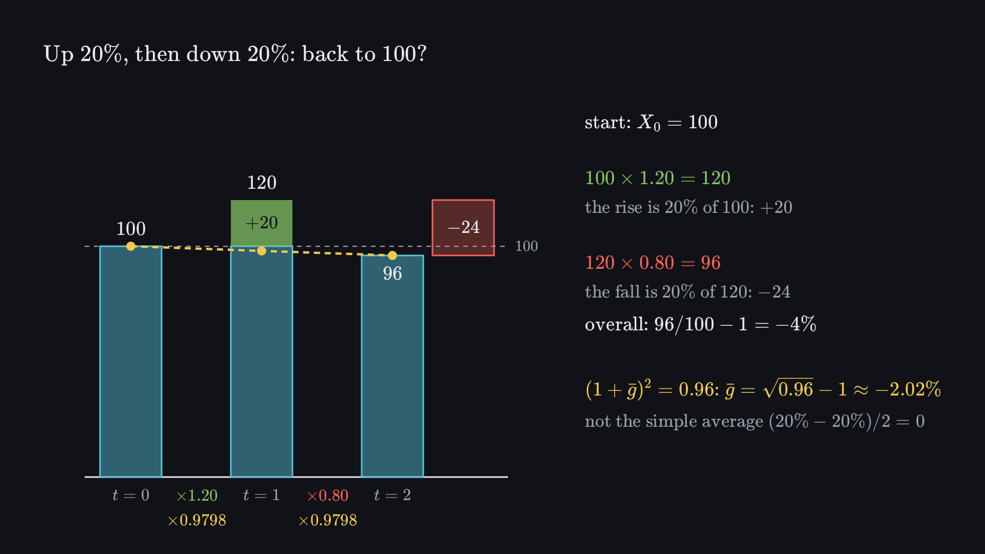
Before it plays Before playing, predict: an index at 100 rises by 20% and then falls by 20%. Where does it end?
4.2Measuring change
Differences subtract, growth factors multiply, logs add
Definition
Differences
ΔXt=Xt−Xt−1: an absolute change, in units of X per period. Δ4Xt=Xt−Xt−4 compares matching quarters; it is not Δ4Xt.
Key formula Definition (2)
Growth factors compound
In words with rate gt=Xt/Xt−1−1, the growth factor 1+gt multiplies the level; gˉ compounds to the observed ratio.
Needs positive levels.
Key formula Identity (3)
Log change
In words the log of the growth factor; log changes add over time. Close to gt only for small rates: 0.20 is growth of e0.20−1≈22.14%.
Needs Xt>0; natural logarithms.
Worked example compounding
Up 20%, down 20%: (1+gˉ)2=0.96, so gˉ≈−2.02% per period, not 0. And 2% a quarter is (1.02)4−1≈8.243% a year, not 8%.
2
Part 2 of 3
Models with memory
What must stay unchanged for the past to inform the future, and does a shock fade or last?
Key terms
stationaritywhite noiserandom walkAR(1)forecast bandSo far a series is one path of a process; autocorrelation measures how it depends on its own past.
Why it matters
Any forecast of unemployment, earnings or an exchange rate rests on a model of persistence. Whether a shock is temporary or permanent decides where the forecast goes, and whether its uncertainty stays bounded.
In this part
- 4.3Weak stationarity: what must stay unchanged
- 4.4White noise and the random walk
- 4.3Choosing a transformation from the model
- 4.4The AR(1) and its special cases
- 4.5Mean, variance and autocorrelation of a stable AR(1)
- 4.5AR(1) forecasts and their uncertainty
- ▶Animation: the forecast returns towards the mean inside a band that levels off
4.3What must stay unchanged
Stationarity: the same probability structure at every date
Key formula Definition (4)
Weak stationarity
In words the same mean and finite variance at every date, and a covariance that depends only on the gap h. Then ρ(h)=γ(h)/γ(0).
Needs finite second moments; it restricts moments, not the whole distribution.
Stationarity lets one stretch of history inform another: the role that iid sampling played in Lecture 3.
Common mistake
Stationary is not flat-looking: long runs above the mean are allowed. Nor is zero autocorrelation enough: Xt∼N(0,t) is uncorrelated but not stationary.
Check
With Zt iid N(0,1), which of 3+Zt, t+Zt and tZt is weakly stationary?
Answer
Only 3+Zt: mean 3, variance 1. t+Zt has mean t; tZt has variance t.
4.4Two building blocks
White noise is the building block; a random walk adds the shocks up
Definition
White noise
The innovation εt is the new component at date t: iid, mean 0, variance σ2>0, independent of the past. Unforecastable in mean, not in spread.
Key formula Result (5)
The random walk accumulates shocks
In words the start plus every shock so far: E[Xt]=x0, but Var(Xt)=tσ2 grows, so it is not stationary.
Needs a fixed start x0 and iid mean-zero shocks.
Result what a walk implies
- Every shock carries into every later level: a random walk has no restoring force.
- Corr(Xt,Xt−h)=(t−h)/t depends on the date: there is no stationary ACF.
- The forecast of Xt+h is Xt, with error variance hσ2.
- With drift d, the mean is x0+td and ΔXt=d+εt.
Common mistake
“It will come back, because its mean is constant.” The constant mean is an average across possible paths at one date; it does not pull a path back. The best forecast is today’s level.
4.3Detrend or difference
Detrend or difference? The model decides
| Model | Transformation | What is left |
|---|---|---|
| Xt=a+bt+Ut | subtract the trend | Ut, stationary |
| Xt=Xt−1+εt | first difference | ΔXt=εt |
| Ut, already white noise | a difference too many | lag-one correlation −21 |
Result over-differencing
Vt=Ut−Ut−1 has variance 2σ2 and lag-one covariance −σ2: the transformation created the correlation.
Common mistake
Fitting a straight line to a random walk does not make what is left stationary.
Check
Can a log transformation remove the growing variance of a Gaussian random walk that takes negative values?
Answer
No: the log is not even defined at negative values. The model justifies the first difference.
4.4Autoregression
One recursion: shocks that vanish, last for ever, or fade
Key formula Definition (6)
The AR(1) model
In words an intercept, plus ϕ times yesterday, plus a new shock. An AR(p) adds lags up to Xt−p.
Needs white-noise shocks; a stable solution needs ∣ϕ∣<1.
| Restriction | Model | A shock … |
|---|---|---|
| c=0, ϕ=0 | white noise | vanishes at once |
| c=0, ϕ=1 | random walk | lasts for ever |
| c=d, ϕ=1 | walk with drift | lasts, around a drifting mean |
| ∣ϕ∣<1 | stable AR(1) | fades: 1, ϕ, ϕ2,… |
Check
Compare Xt=2+Xt−1+εt with Yt=2+0.5Yt−1+εt. Which has a stationary long-run mean?
Answer
Only Y: μ=2+0.5μ gives μ=4. X is a walk with drift 2; its mean x0+2t keeps rising.
4.5The stationary AR(1)
A stable AR(1): the intercept is not the mean
Key formula Result (7)
Stationary mean and variance
In words expectations of the recursion give μ=c+ϕμ; variances give v=ϕ2v+σ2.
Needs ∣ϕ∣<1, the stationary solution.
Key formula Result (8)
Autocorrelation of an AR(1)
In words the new shock is independent of the past, so γ(h)=ϕγ(h−1); and ρ(1)=ϕ.
Exact ρ(h): ϕ=0.8 solid, ϕ=−0.8 dashed.
Check
Xt=3+0.6Xt−1+εt with innovation variance 2: find μ, v and ρ(2).
Answer
μ=3/0.4=7.5; v=2/0.64=3.125; ρ(2)=0.36.
4.5Forecasting
Forecast the centre, then state the uncertainty
Key formula Result (9)
AR(1) forecast and error variance
In words the mean plus ϕh times today’s deviation. The error is the sum of the h unseen shocks, weighted 1,ϕ,…,ϕh−1.
Needs information through t and known parameters; normal shocks for the interval ±1.96Vh.
Result as the horizon grows
The forecast tends to μ and Vh to the stationary variance: the band levels off. For a random walk the forecast stays at Xt and hσ2 grows without limit.
Worked example a worked forecast
μ=10, ϕ=0.8, σ2=1, and today Xt=15.
Xt+1∣tXt+2∣tV2=10+0.8(5)=14=10+0.82(5)=13.2=1+0.82=1.6495% interval: 13.2±1.961.64=[10.69, 15.71].
Why economists care
A forecast is a distribution: report its centre and its band. Estimating μ, ϕ and σ2 from data adds further uncertainty.
![Final frame: a time plot with the mean μ = 10 dashed. An illustrative past path rises to X_t = 15. From there the forecast centre falls towards 10 (14, 13.2, 12.56, …), inside a shaded 95% band that widens and then levels off between dashed limits 10 ± 3.27; two steps ahead, a yellow bracket marks [10.69, 15.71]. Three simulated green paths continue from 15, and one first rises to about 15.6. Beside it: μ = 10, φ = 0.8, σ² = 1, X_t = 15; X̂_{t+h|t} = 10 + 0.8^h(15 − 10) = 14, 13.2, 12.56, … → 10; V₂ = 1 + 0.8² = 1.64; 13.2 ± 1.96√1.64 = [10.69, 15.71]; V_h → 1/(1 − 0.8²) ≈ 2.78, so the band levels off. The expected deviation shrinks; a realised value can still rise.](media/ar-forecast-end.png?v=b9fd44690f)
Before it plays Before playing, predict: the series stands at 15, above its mean 10. Must the next value be lower? And does the forecast’s uncertainty keep growing?
3
Part 3 of 3
Reversion and spurious correlation
When does movement towards the mean, or a strong correlation between two series, reveal a real mechanism?
Key terms
mean reversionregression to the meanspurious regressioncointegrationSo far a stable AR(1) forecast returns towards μ; a random walk’s stays at today’s level while its variance grows.
Why it matters
Programmes that select extreme cases, such as tutoring the lowest scorers or treating road sites after unusually many accidents, can show before–after improvements with no effect. Regressing one trending level on another can give a high fit and a small p-value with no relationship at all.
In this part
- 4.6Mean reversion is a property of the expected path
- ▶Animation: why extreme first scores drift back on retest
- 4.6Regression to the mean, and what it means for programmes
- 4.7Independent random walks can correlate strongly
- 4.7Before trusting a correlation between two series
4.6Mean reversion
Mean reversion describes the expected path, not the next value
Definition
Mean reversion
In a stable AR(1) the expected deviation after h periods, ϕh(Xt−μ), tends to zero. Next period’s expected change is
E[Xt+1−Xt∣Ft]=(ϕ−1)(Xt−μ)which is negative when today is above the mean.
Worked example half-life
The expected deviation halves when ϕh=1/2, so h1/2=log(1/2)/logϕ. At ϕ=0.8 that is about 3.11 periods.
Check
μ=0, ϕ=0.8, and today’s value is 5. Must the next value be below 5?
Answer
No. The forecast is 4, but Xt+1=4+εt+1 exceeds 5 whenever the shock exceeds 1. The expected change is −1; the realised change is not restricted.
Common mistake
“It is far above its historical average, so it will fall.” That needs an identified restoring model. A random walk has a constant unconditional mean but no restoring forecast.
![Final frame: a scatter of 300 simulated people, first score S₁ against retest score S₂, with a dashed no-change line S₂ = S₁ and a green conditional-mean line of slope 0.6. A strip of first scores near 30 is highlighted; a sideways yellow curve shows their retest distribution N(38, 8²), with an arrow up from 30 to 38 marked +8. A strip near 80 shows the curve N(68, 8²), with an arrow down from 80 to 68 marked −12. Beside it: S₁ = 50 + A + U₁ and S₂ = 50 + A + U₂, Var(A) = 60 persists and Var(U_i) = 40 is fresh; E[S₂ | S₁ = 30] = 50 + 0.6(30 − 50) = 38, +8 with no programme at all; E[S₂ | S₁ = 80] = 50 + 0.6(80 − 50) = 68; r = 60/(60 + 40) = 0.6, slope 0.6, not 1. Extreme first scores carry unusual noise; the retest draws fresh noise. A before–after gain is not a programme effect.](media/regression-mean-end.png?v=1be84b1182)
Before it plays Before playing, predict: people who scored 30, well below the mean 50, are retested with no help at all. What should their average retest score be?
4.6Regression to the mean
Selecting extreme first scores also selects favourable noise
Key formula Result (10)
Regression to the mean
In words a score is μ plus a lasting part (variance τ2) plus fresh noise (variance ω2); the retest keeps the share r of the first deviation.
Needs the Gaussian model Sk=μ+A+Uk, all parts independent.
Result two extremes
Pure guessing: the top scorers’ expected retest is the mean. No new noise: no regression at all.
Why economists care
A school tutors its lowest scorers. With μ=50 and r=0.6, a first score of 30 retests at 38 on average, with no effect at all. A before–after gain mixes an effect, regression to the mean, a common trend and noise. Ask what the same selection gives without treatment (Lecture 5).
The same form as the AR(1) forecast, a different mechanism: a lasting component measured twice, and selection on the first measurement.
4.7Back to the opening question
Back to 0.71: independent random walks can correlate strongly
Worked example two independent walks
Xt=Xt−1+εt and Yt=Yt−1+ηt, both from 0, with independent N(0,1) shocks. An early positive shock lifts X for many later dates; an unrelated early shock may do the same for Y. Across one realised sample, their levels then move together.
Neighbouring dates share shocks, so T date pairs are not T independent pieces of information.
Result the opening question
(c). The generator did not link the series. Nor does a longer sample help: levels correlations stay widely spread across independent pairs.
The notes’ lab: 200 prespecified pairs of independent walks, T=100.
| Levels (Xt,Yt) | ∣r∣>0.5 in 85 of 200 pairs |
|---|---|
| Changes (ΔXt,ΔYt) | ∣r∣>0.5 in 0 of 200: independent iid pairs, correlation zero |
4.7Carry the question through
A high coefficient does not choose its own explanation
Definition
Spurious regression
Misleading evidence of a relationship when unrelated persistent, nonstationary levels are regressed on one another, using inference designed for a different error structure.
Result four sources of a high coefficient
- A common driver of both series.
- Two deterministic trends, such as Xt=t+εt and Yt=2t+ηt.
- A search across many pairs that selects an extreme one.
- Nonstationary levels, which align even when the processes are independent.
Common mistake
“The p-value is tiny, so the relation is real.” iid correlation tests and regression standard errors are wrong for random-walk levels; a small p-value from the wrong reference distribution is not reassuring.
Transform because the model says so. Differencing changes the question and can remove a real long-run relation: some nonstationary series have a stationary combination, called cointegration.
Review · How the ideas connect
Describe, model the memory, then interpret through the model
Part 1 · Describe
Part 2 · Model
Part 3 · Interpret
Xt=c+ϕXt−1+εt
Review · Summary sheet
What to take away: the terms and the ten formulas
Key terms
1 Order, units and change
Time series and process ordered data; the process {Xt} is their probability model, and we observe one path.
Differences ΔXt=Xt−Xt−1; Δ4Xt compares matching quarters.
growth factor 1+gt multiplies the level; rates compound, they do not add.
2 Models with memory
White noise the new shock εt: iid, mean 0, variance σ2.
random walk Xt=Xt−1+εt: every shock is permanent and the variance tσ2 grows.
forecast the expected Xt+h given information at t; Vh is its error variance.
3 Reversion and spurious correlation
Mean reversion the expected deviation ϕh(Xt−μ) shrinks to zero when ∣ϕ∣<1.
regression to the mean selecting extreme noisy scores selects favourable noise too, so retests move towards the mean.
Spurious regression misleading evidence of a link between persistent levels, from iid-style inference.
Key formulas
1 Order, units and change
2 Models with memory
3 Reversion and spurious correlation
Review · Remember
Keep the order, model the memory, question the pattern
Result the opening question
(c). The series were independent random walks. Their levels share shocks across dates, so a correlation of 0.71 is unremarkable; their changes are independent pairs.
Remember
- Keep the dates, units and information set: differences subtract, growth factors compound, logs add.
- In Xt=c+ϕXt−1+εt, ∣ϕ∣<1 makes shocks fade and forecasts return to μ inside a band that levels off; ϕ=1 makes them last.
- Reversion and strong level correlations can arise with no mechanism: ask what the same model or selection gives without the claimed link.
Before next time
- Notes 4.1–4.7 with the worked solutions.
- The four labs: scales, the AR(1), retest scores and independent walks.
- Rework the forecast with μ=20, ϕ=−0.5, σ2=4, Xt=24.
Next · Lecture 5
Causal inference. A before–after gain after selection, or a correlation between two series, is not an effect. Which comparison identifies one?