A connected route from probability to causal reasoning
The learning route
These five topics form a connected course in probability and statistics. Each changes the question we ask of data: what can happen, how measurements vary, how samples inform a population, what time dependence changes, and which comparison identifies an effect.
Each topic has a lecture: present its slides in the browser, or read the same slides as a PDF with every step shown. Within each topic, read chapters in order. Topic 2 places expectation and variance before normal standardization so that its subtraction and division have a clear meaning. Topic 3 treats single, independent and paired designs explicitly. The later topics revisit the assumptions behind earlier formulas.
How to study a derivation
Name the object. State the variable, event, population or causal target before using a formula.
Read the assumptions. Equal weights, independence, finite moments, stationarity and conditional independence serve different purposes.
Follow each step. The notes distinguish definitions, algebraic identities and results that need assumptions.
Predict, then inspect. Use a control when it changes a denominator, weighting scheme, sampling distribution or model. Explain why the result moves.
Rework the exercises. Attempt the question before opening its solution. Check both the numerical result and its interpretation.
The contents menu opens topics and chapters directly. All notes gives a continuous reading view. Each topic has a static print view with solutions expanded; the PDF contains the complete course. Mathematical notation is typeset locally, and the static notes remain readable without JavaScript.
1.1 Probability basics
Outcomes, sets and a consistent probability model
1.1.1 Outcomes, events and a probability model
A probability question needs a precise description of what would make its answer “yes”. A die roll produces one face, but “the result is even” is true for three faces. A bulb has one realised lifetime, but “it survives at least ten hours” is true for many possible lifetimes. Representing each question as a set lets us calculate with these different kinds of uncertainty using the same rules.
Definition. An outcome is one possible result. The sample spaceΩ is the set of all possible outcomes considered by the model. An eventA is a subset of Ω: the outcomes for which a specified statement is true.
Write ω∈Ω for an individual outcome and A⊆Ω for an event. If the realised outcome belongs to A, the event occurs. Membership is a yes-or-no statement about that outcome. The probability P(A) describes uncertainty before learning the outcome. Different events may occur in the same experiment: one die result can be both even and prime.
Definition. The event spaceF is the collection of events to which probabilities are assigned. A probability functionP assigns each event A∈F a number P(A) between 0 and 1, consistently with the axioms in Section 1.1.4.
The three objects (Ω,F,P) form a probability model. They specify what could happen, which events are allowed, and how much probability each event receives. The letter P names a function; the parentheses in P(A) say which event is its input. A fair die and a loaded die can have the same possible outcomes and the same events, but different probability functions.
The unit scale makes comparisons consistent: probability 0.25 represents one quarter of the whole model's mass, or 25%. It does not promise that exactly one quarter of every short sequence of experiments will realise the event. A probability assignment and an observed frequency are different objects.
Formal precision: allowed events
An event space is a sigma-algebra: it contains Ω, complements of its events, and countable unions of its events. “Closed under” these operations means their results remain in the collection. This ensures that combining allowed questions produces another allowed question.
In our finite models we allow every subset, including the empty set and the whole space. An event is measurable here when it belongs to the chosen event space, so the model assigns it a probability. In continuous models the usual measurable collection contains intervals and their countable combinations; it need not contain every imaginable subset. This technical restriction does not prevent us from asking the lifetime questions considered here.
Before calculating: Name the experiment, describe one outcome, and identify all outcomes that make the event true. Then ask what probability weights the model supplies.
1.1.2 Three sample spaces
A die: fairness supplies the probability weights
For one roll of a six-sided die, consider three questions: is the result six, even, or prime?
ΩAC={1,2,3,4,5,6},={6},B={2,4,6},={2,3,5}.
Here A means “six”, B means “even”, and C means “prime”. Braces collect the outcomes belonging to a set. The number 2 is an outcome; {2} is the event containing that outcome. Rolling it makes both B and C occur.
A fair die assigns probability 1/6 to each face. Adding the three distinct even-face probabilities gives
P(B)=61+61+61=∣Ω∣∣B∣=63=21.
The counting fraction works because the outcomes are equally likely. Each selected face contributes the same weight. For any finite model, the general calculation is to add the weights of the distinct outcomes in the event; the fair model makes those weights equal.
For a concrete hypothetical loaded die, give each of faces 1 to 5 probability 0.1, and give face 6 probability 0.5. These nonnegative weights sum to 1. The event B is still {2,4,6}, but now
P(B)=0.1+0.1+0.5=0.7.
The prime event C still has three faces, yet its probability is 0.1+0.1+0.1=0.3. Equal numbers of outcomes need not mean equal probability. Loading changes the weights, not whether a face is even or prime.
Fair die, event E={2,4,6}: P(E)=3/6=1/2. For even or prime the selected set is {2,3,4,5,6}, with probability 5/6; for even and prime it is {2}, with probability 1/6.
First select the faces belonging to the event. Then count them under the fair-die assumption. Event labels inside the interaction refer to its current selections.
A coin: an event space is a set of sets
Model one toss as having two recorded outcomes: H for heads and T for tails. This model excludes other recorded results. Then
ΩF={H,T},={∅,{H},{T},{H,T}}.
The four events are neither outcome, heads, tails, and either outcome. The symbol ∅, read “the empty set”, denotes an impossible event; the whole sample space is a certain event. Notice the two levels of braces: {H} contains an outcome, while F contains events. Each of the two outcomes can be included or excluded, giving 22=4 events.
Enumerating events requires no fairness assumption. We could assign heads any probability p between 0 and 1, then assign tails 1−p. Here p, read “pee”, is a model parameter. The probability of heads becomes 1/2 only when fairness supplies that value.
A bulb: intervals replace lists of outcomes
To ask whether a bulb fails early or lasts through a required period, model its finite lifetime in hours by a nonnegative real number t, with Ω=[0,∞). For example, consider
{t:0≤t≤100},{t:t≥10},{t:30≤t≤40}.
These mean at most 100 hours, at least 10 hours, and between 30 and 40 hours. The inequalities determine membership: a realised lifetime of 35 hours belongs to all three events; a lifetime of 150 hours belongs only to the second.
The sample space contains infinitely many lifetimes. A finite counting fraction cannot supply an interval's probability, and no uniform probability exists over this entire unbounded half-line. Nor does a longer interval automatically have more probability than a shorter one elsewhere. A lifetime distribution supplies the weights; its construction is developed in the next topic.
An event can be an interval
Each thick segment is the set of lifetimes satisfying the statement. Filled endpoints are included. The arrow in the middle row continues beyond every finite lifetime. A segment’s length alone does not give its probability: that requires a lifetime distribution.
Separate two questions: Is a given lifetime in the interval? How much probability does the model assign to that interval? The first follows from the inequalities; the second needs a distribution.
1.1.3 “Not”, “and” and “or”
Set operations let us build a new question from existing questions. They first determine which outcomes belong to the event; probabilities are assigned afterwards.
Statement
Event
Membership requirement
Not A
Ac
Inside Ω, outside A.
A and B
A∩B
Inside both sets.
A or B
A∪B
Inside at least one, including both.
A, but not B
A∖B
Inside A, outside B.
Probability uses inclusive “or”. An outcome in both events belongs to their union once. Events are disjoint, or mutually exclusive, when A∩B=∅; then they cannot occur together.
For the die, B∩C={2} and B∪C={2,3,4,5,6}. The complement of even is Bc={1,3,5}. These statements concern membership and remain true for a loaded die.
A picture of “and”, “or” and “not”
The left oval is the even event B; the right oval is the prime event C. Only 2 lies in both. The union contains every labelled outcome except 1. The complement of even contains 1,3,5. Oval areas do not encode probabilities: the labelled outcomes determine membership.
Before adding probabilities: List the distinct included outcomes. Does any outcome satisfy both statements? “Even or prime” includes the face 2 once, although it answers both questions.
For a separate pair of events, suppose P(A)=0.25, P(B)=0.15, and P(A∩B)=0.05. Their four disjoint regions have probabilities 0.20 for A only, 0.05 for both, 0.10 for B only, and 0.65 for neither. Their total is 1. We obtain these values by keeping the overlap in its own region, then subtracting it from each marginal; Section 1.1.5 justifies that accounting.
Region
A only
Both
B only
Neither
Mass
0.20
0.05
0.10
0.65
The union comprises the first three regions: 0.20+0.05+0.10=0.35. Not A comprises the last two: 0.10+0.65=0.75.
A quantitative diagram divides probability mass into non-overlapping regions. Select “and”, “or” or “not” and identify which regions the statement includes before reading the answer.
In a quantitative diagram, area or width is deliberately scaled to probability. A unit square can represent the whole model, with total probability 1; a region occupying one quarter then represents probability 0.25. An ordinary Venn diagram need only represent membership and overlap: its drawn areas need not equal probabilities. Read the diagram’s scale before interpreting its geometry.
1.1.4 The axioms of probability
The axioms impose consistency on probability assignments. They prohibit negative mass, fix the total, and specify how distinct parts combine. They do not choose the weights of a particular die or lifetime model.
Axiom 1 — nonnegativity. For every allowed event, P(A)≥0.
Axiom 2 — normalisation.P(Ω)=1.
Axiom 3 — countable additivity. For pairwise disjoint events A1,A2,…,
P(i=1⋃∞Ai)=i=1∑∞P(Ai).
“Pairwise disjoint” means Ai∩Aj=∅ whenever i=j. The subscript labels the events; it is not part of their probability. For a finite collection, the same rule uses a finite union and sum. Distinct regions may be added because no outcome's probability mass is counted twice.
For example, two disjoint events with probabilities 0.2 and 0.1 have union probability 0.3. Disjoint events with masses 0.1 and 0.01 similarly have union probability 0.11. These calculations use disjointness, which prevents double counting; they require no equal-outcome assumption.
One immediate consequence is P(∅)=0. The disjoint union Ω∪∅ is still Ω. Additivity therefore gives P(Ω)=P(Ω)+P(∅); subtracting P(Ω)=1 leaves zero.
The converse needs care: an event with probability zero need not be the empty set. Continuous models can assign zero probability to a single exact value. The empty set is logically impossible; a zero-probability event is a statement about the model's mass assignment.
We now have a consistent way to add disjoint pieces. The next step is to decompose more complicated events into such pieces, then use the same axiom to derive useful rules.
1.1.5 Four rules, derived from the axioms
Complement rule
Goal: Express the probability outside A using P(A).
Proposition.P(Ac)=1−P(A).
Before playing, decide which axiom makes the total 1 and which one lets you add. The animation then derives the rule in four steps.The animation’s final frame. Its numbered steps describe how the picture is built.
A takes 0.25 of the area. Everything else in Ω is Ac.
Together they make Ω, so P(A∪Ac)=P(Ω)=1 by Axiom 2.
They do not overlap, so P(A∪Ac)=P(A)+P(Ac) by Axiom 3.
Equate the two expressions: P(A)+P(Ac)=1.
Rearrange: P(Ac)=1−P(A)=1−0.25=0.75.
Set identity. Every outcome is in A or outside it, so A∪Ac=Ω and A∩Ac=∅.
Disjoint additivity and normalisation.P(A)+P(Ac)=P(Ω)=1.
Rearrangement. Subtract P(A) from both sides.
If an event has probability 0.25, its complement has probability 1−0.25=0.75. Also, nonnegativity of the complement gives P(A)≤1. Together with Axiom 1, this proves the familiar bound 0≤P(A)≤1.
The rule is useful when “not” is easier to describe than the desired event. For a bulb, “lasts more than 100 hours” is the complement of “lasts at most 100 hours.” The endpoint belongs to the latter event, so the two events are disjoint and exhaustive.
Union rule: remove the duplicated overlap
Proposition.P(A∪B)=P(A)+P(B)−P(A∩B).
Adding the two marginal probabilities counts their intersection twice. Here “marginal” means the probability of each event considered separately, regardless of whether the other occurs. The derivation makes the required subtraction precise.
Play to see each term of P(A∪B)=P(A)+P(B)−P(A∩B) come from the picture. The areas are drawn to scale, so every probability is an area.The animation’s final frame. Its numbered steps describe how the picture is built.
Ω has area 1. The events A and B are drawn to scale.
Paint A:P(A)=0.25 includes the overlap.
Paint B: the overlap is now painted twice, so 0.25+0.15=0.40 is too large.
Lift off the second copy of the overlap. It becomes the subtracted term, −P(A∩B)=−0.05.
Outline the union: each point is counted once, so P(A∪B)=0.35.
Disjoint decomposition of A.A=(A∖B)∪(A∩B). Additivity gives P(A)=P(A∖B)+P(A∩B).
Rearrangement.P(A∖B)=P(A)−P(A∩B).
Disjoint decomposition of the union.A∪B=(A∖B)∪B. These parts are disjoint, so additivity gives P(A∪B)=P(A∖B)+P(B).
Substitution. Insert Step 2 into Step 3 to obtain the proposition.
With the probabilities from Section 1.1.3, the rule gives 0.25+0.15−0.05=0.35. Adding the three included regions, 0.20+0.05+0.10, gives the same answer. The overlap is subtracted once because the desired union must still include it once.
Union bound
Proposition.P(A∪B)≤P(A)+P(B).
Union rule: the union is the sum minus P(A∩B). Nonnegativity: this subtracted quantity is at least zero. Subtraction cannot increase the sum, which proves the bound. Equality holds when the overlap has probability zero; disjoint events guarantee that condition. The bound may exceed 1, so min{1,P(A)+P(B)} is a tighter upper bound when necessary. Here min means “the smaller of”.
Logical consequence, or monotonicity
Proposition. If B⊆A, then P(B)≤P(A).
Set inclusion. If B occurs, A must occur: every outcome of B is in A.
Disjoint decomposition and additivity.A=B∪(A∖B), hence P(A)=P(B)+P(A∖B).
Nonnegativity.P(A∖B)≥0, so P(A)≥P(B).
Adding a requirement restricts an event to a subset and cannot increase its probability. For the fair die, “six” implies “even”. In Section 1.1.2 these were A={6} and B={2,4,6}, so that inclusion gives P(A)=1/6≤P(B)=1/2. The letters do not determine which set is larger; identify the actual inclusion before applying the rule.
The same relationship holds for the hypothetical loaded die: 0.5≤0.7. Its numerical probabilities change, but the logical implication does not. Set relationships constrain every valid probability assignment.
1.1.6 Exercises with worked reasoning
For each question, identify the outcomes first. State the probability assumption, choose a rule, and explain why its conditions hold. Distinguish an exact answer from a bound: knowing that an event lies inside another can restrict its probability without determining it.
Exercise 1. For the fair die with B={2,4,6}, C={2,3,5}, find the probabilities of “even and prime”, “even or prime”, and “not even”. Explain why adding P(B)+P(C) alone is incorrect.
Solution
Intersection and fairness. Only 2 belongs to both sets: P(B∩C)=1/6.
Union rule.P(B∪C)=3/6+3/6−1/6=5/6. The naive sum counts the face 2 twice.
Complement rule.P(Bc)=1−3/6=1/2. Its outcomes are {1,3,5}.
Exercise 2. Given P(A)=0.25, P(B)=0.15, P(A∩B)=0.05, recover all four disjoint regions. Find the probability of neither event and check the union bound.
Solution
Disjoint decomposition.A-only has mass 0.25−0.05=0.20; B-only has mass 0.15−0.05=0.10. Both has mass 0.05.
Additivity. The union has mass 0.20+0.10+0.05=0.35.
Complement rule. Neither is (A∪B)c, with mass 1−0.35=0.65. All four masses are nonnegative and sum to 1.
Union bound.0.35≤0.25+0.15=0.40. The difference is exactly the overlap 0.05.
Exercise 3. Suppose a hypothetical bulb-lifetime model assigns probability 0.8 to lasting at most 100 hours. Could the probability of lasting between 30 and 40 hours be 0.9? Does the supplied probability determine the exact answer?
Solution
Inclusion.[30,40]⊆[0,100].
Monotonicity and nonnegativity.0≤P(30≤t≤40)≤0.8. Therefore 0.9 is inconsistent.
What remains unspecified. The model has not said how the mass within [0,100] is distributed. We have a bound, not an exact probability. A fuller lifetime distribution is required.
These rules combine probabilities within a fixed model. The next chapter considers what changes when we learn that a particular event has occurred.
1.2 Conditional probability
Information, reference groups and weighted probabilities
1.2.1Information changes the question
A probability describes uncertainty relative to the information available. Before learning anything else, we consider the whole sample space. After learning that an event occurred, we consider only possibilities consistent with that event. Conditional probability expresses this change of reference group: among the possibilities compatible with what we know, how much probability belongs to the event we are asking about?
Consider a family with two children. Use a toy model in which each child has a boy or girl outcome, each with probability 1/2. Assume the two outcomes are independent: knowing one does not change the probabilities for the other. Order the children from older to younger, writing b for boy and g for girl. These assumptions define the exercise; they are not demographic claims. The sample space is
Ω={(b,b),(b,g),(g,b),(g,g)}.
Independence gives each ordered pair probability (1/2)(1/2)=1/4. The mixed pairs are distinct: (b,g) has an older boy, while (g,b) has an older girl. Let A be “two boys” and B be “at least one boy.” Then
AB={(b,b)},={(b,b),(b,g),(g,b)}.Before playing, predict: once you know there is at least one boy, is two boys more or less likely than 1/4?The animation’s final frame. Its numbered steps describe how the picture is built.
Four equally likely families: each has probability 1/4.
Two boys is one of them: P(A)=1/4.
Learn B, that there is at least one boy: (g,g) is ruled out.
The three that remain share the whole, a third each, so P(A∣B)=(1/4)/(3/4)=1/3.
No family changed; only the group we compare with did.
Specify how the information is obtained. Choose a family at random from this model, check whether it has at least one boy, and retain it exactly when B is true. This procedure excludes (g,g) without favoring one of the three retained outcomes over another. Of the retained probability 3/4, the part belonging to two boys is 1/4. Therefore
P(A∣B)=3/41/4=31.
Before screening, the probability of two boys was 1/4; within the screened group it is 1/3. No family has changed. We have changed the group within which the fraction is calculated.
Different information procedures give different answers
If we instead learn that the older child is a boy, only (b,b) and (b,g) remain. They are equally likely, so the probability of two boys is 1/2. “The older child is a boy” and “at least one child is a boy” are different events, even though both imply that the family has a boy.
Now choose one of the two children at random, independently of the family’s outcomes, and observe that the selected child is a boy. A two-boy family always produces that observation; a mixed family produces it only half the time. Mixed families therefore receive less weight than two-boy families among observations of a boy. To count explicitly, pair each of the four family outcomes with either choice of child. There are eight equally likely family–child pairs. Four produce a boy: two from (b,b), one from (b,g), and one from (g,b). Two of those four come from a two-boy family, giving 2/4=1/2.
The statement we heard is not enough to justify a calculation if its reporting procedure is unspecified. In particular, a parent choosing which child to mention need not reproduce either procedure above. First define what was checked or observed; then identify the outcomes and weights consistent with that information.
Ordered outcome
At least one boy
Older child a boy
(b,b)
Retained
Retained
(b,g)
Retained
Retained
(g,b)
Retained
Excluded
(g,g)
Excluded
Excluded
With independent children’s outcomes and equal boy/girl probabilities, these conditioning events give probabilities of two boys 1/3 and 1/2, respectively.
Compare screening for at least one boy with knowing the older child is a boy under the same family model. Predict which outcomes remain before inspecting the answer.
1.2.2Restriction, normalization and the definition
Counting retained outcomes worked above because the relevant cases were equally likely. The general definition uses their probability weights instead. Let A be the event we want to assess and B the information on which we condition.
Definition. For events A and B, provided P(B)>0,
P(A∣B)=P(B)P(A∩B).
The numerator is not P(A): some outcomes in A may be incompatible with the information. We retain only the intersection A∩B, meaning outcomes where both events occur. The denominator is not the probability of the whole sample space: our reference group is now B. We divide the retained part of A by the probability of that entire reference group.
Why divide by the probability of the information?
Restriction. Exclude outcomes outside B. The retained part of A is A∩B, with its original probability P(A∩B).
Preserve relative weights. Apply one common multiplier c to all retained probabilities. If one retained part originally had twice the probability of another, it must still have twice the probability after conditioning.
Normalize. The entire retained group must have conditional probability one. Thus cP(B)=1, which gives c=1/P(B).
Apply the multiplier. The conditional probability of A is cP(A∩B)=P(A∩B)/P(B).
Before playing, predict: when B is stretched to fill the whole square, what share of it will the overlap fill?The animation’s final frame. Its numbered steps describe how the picture is built.
The model: P(A)=0.2,P(B)=0.6 and P(A∩B)=0.1.
Learn that B happened: everything outside B is ruled out.
B swells to fill the square. Every part of it grows by the same factor, 1/0.6, so the overlap keeps its share of B:1/6.
So P(A∣B)=P(A∩B)/P(B)=0.1/0.6=1/6, and the two parts of B still add to 1.
Shrinking back multiplies by P(B):P(A∩B)=P(A∣B)P(B)=1/6×0.6=0.1.
This process is called renormalization: restoring a total of one after restriction. For example, suppose P(A)=0.2, P(B)=0.6 and P(A∩B)=0.1. The intersection contributes probability 0.1, and the rest of B contributes 0.6−0.1=0.5. Write Ac, read “A complement,” for not A. Conditioning scales these two retained parts by 1/0.6:
P(A∣B)P(Ac∣B)=0.60.1=61,=0.60.5=65.
The rescaled parts add to one. The original probability P(B) remains 0.6; the new probability P(B∣B) is one. Conditioning creates a different probability assessment rather than overwriting the original one.
Keep the information group, then rescale it
Whole model
P(A∩B)=0.10 inside P(B)=0.60.
Within the retained group
0.10/0.60=1/6 of the new total.
In the whole-model diagram, the dashed boundary encloses B; its two lower regions have total mass 0.60. Only the lower-left piece also belongs to A. The retained-group diagram redraws the retained mass as a new whole: the event of interest occupies one sixth. Conditioning changes the reference group, not which outcomes lie in the intersection.
The product rule reverses the rescaling
If P(A∣B) describes the fraction inside B, multiplying by the size of B restores its share of the original whole:
Product rule. When P(B)>0,
P(A∩B)=P(A∣B)P(B).
Conditional definition. Begin with P(A∣B)=P(A∩B)/P(B).
Multiply both sides by the denominator. This gives the displayed product rule.
The left side is a joint probability: the probability that both events occur. It equals the probability of belonging to B, multiplied by the fraction of that group also in A. Replacing P(A∣B) with P(A) would be an additional claim that the information B leaves the probability of A unchanged. The next chapter identifies that condition as independence.
Definition or starting axiom?
The elementary approach here defines conditional probability by the ratio and derives the product rule by rearrangement. Other foundations take a multiplication relationship as a starting point for conditional probability. This distinction does not change the calculations for positive-probability conditioning events.
The probability rules continue to hold
Keep B fixed with P(B)>0. Nonnegativity and the fact that A∩B is contained in B give
0≤P(A∣B)≤1.
The reference group is certain under its own condition, while its complement is excluded:
P(B∣B)P(Bc∣B)=1,=0.
For events A1,A2,… that are mutually exclusive withinB, conditional probabilities add. “Within B” means that no outcome in B belongs to two of these events, even if they overlap outside B.
P(i⋃Ai∣B)=i∑P(Ai∣B).
The proof uses the earlier additivity rule on the disjoint intersections with B, then divides every term by the same P(B). The notation ⋃iAi means “the union of the A sub i events,” and ∑i means “sum over i”; the list may be finite or countably infinite. In particular, the complementary parts inside B satisfy
P(Ac∣B)=1−P(A∣B).Why require a positive-probability condition?
If P(B)=0, the ratio divides by zero and is undefined. An exact value in a continuous model can have probability zero without being logically impossible. Conditioning on such values requires other constructions; the elementary event ratio cannot supply the answer.
1.2.3Reversing the condition changes the denominator
“Among cases in B, how many are in A?” asks for P(A∣B). “Among cases in A, how many are in B?” asks for P(B∣A). These are different questions about the same joint event. Provided both conditioning probabilities are positive,
P(A∣B)P(B∣A)=P(B)P(A∩B),=P(A)P(A∩B).
The intersection is symmetric: “A and B” describes the same outcomes as “B and A.” The conditional calculation is not symmetric, because it divides by a different reference group. Interchanging the letters therefore does not justify keeping the same value.
Represent the preceding probabilities using a hypothetical group of 100 cases:
Four disjoint groups with the stated probability weights
Event
B
Bc
Total
A
10
10
20
Ac
50
30
80
Total
60
40
100
Before playing, predict: are P(A∣B) and P(B∣A) equal here? Both count the same 10 cases in A∩B.The animation’s final frame. Its numbered steps describe how the picture is built.
A hypothetical group of 100 cases: 20 in A,60 in B and 10 in both.
Among the 60 cases in B,10 are in A:P(A∣B)=10/60=1/6.
Gather the 20 cases in A: half of them, 10, are in B, so P(B∣A)=10/20=1/2.
The same 10 cases, compared with different groups, give different answers.
Conditioning on B selects the column containing 60 cases. Its 10 cases in A give P(A∣B)=10/60=1/6. Conditioning on A selects the row containing 20 cases. Its 10 cases in B give P(B∣A)=10/20=1/2. The 10 cases in both events have not changed; the group used to interpret them has.
A verbal example makes the distinction clear. Suppose most students in a hypothetical population are Democrats. That need not mean that most Democrats in that population are students: the Democrat group may be much larger and include many nonstudents. One fraction uses the student total; the other uses the Democrat total. A larger denominator makes the fraction smaller for the same overlap, but group sizes and overlap are both needed to calculate how small.
Reverse conditionals can coincide in particular models. For example, if the two reference groups have the same positive probability, the equal numerators and denominators give equal answers. Equality in one example is not a general rule. Bayes’ rule in the next chapter connects the two directions while accounting for their different denominators.
1.2.4Recovering an overall probability from groups
Conditioning isolates a group. Often we need the reverse task: combine the probabilities within several groups to recover a probability for the whole population. This requires knowing both each group’s internal rate and its share of the population.
A partition divides the sample space into groups that are exhaustive and mutually exclusive. Exhaustive means every possible outcome belongs to a group; mutually exclusive means no outcome belongs to more than one. For two groups B1 and B2,
B1∪B2=Ω,B1∩B2=∅.
Law of total probability. For this partition, provided both group probabilities are positive,
P(A)=P(A∣B1)P(B1)+P(A∣B2)P(B2).
The event A can occur through either group. First calculate the share of the whole population that belongs to a group and satisfies A; then add those disjoint contributions.
Exhaustiveness. Every outcome in A belongs to a group, so A=(A∩B1)∪(A∩B2).
Disjointness and additivity. These two pieces do not overlap, so P(A)=P(A∩B1)+P(A∩B2).
Product rule. Substitute P(A∩Bi)=P(A∣Bi)P(Bi) for each group.
Break the target event into disjoint pieces
The three columns form a partition: every outcome belongs to exactly one group. The hatched event A is the union of the separate pieces A∩B1, A∩B2 and A∩B3. To recover each piece’s probability, multiply its within-group rate by the group’s probability; then add. This is a membership sketch, so drawn sizes are not assigned probabilities.Before playing, predict: is P(A) the plain average of the two group rates, 1/6 and 1/4?The animation’s final frame. Its numbered steps describe how the picture is built.
Split Ω into two groups, B and Bc, of sizes 0.6 and 0.4: every case is in exactly one.
Inside each group A has its own rate: P(A∣B)=1/6 and P(A∣Bc)=1/4.
Each rate times its group size is an area: 1/6×0.6+1/4×0.4=0.1+0.1=0.2.
Averaging the two rates would treat the groups as equal and give about 0.208. The group sizes are the weights.
Why the group probabilities are weights
The rate P(A∣Bi) is measured within group Bi, where that group is treated as the whole. Multiplying by P(Bi) converts it into a share of the original population. For an exhaustive, disjoint partition, these weights add to one. A large group contributes more than a small group with the same internal rate; simply averaging the rates would implicitly assign equal population shares.
Return to the table above. The groups B and Bc contain respectively 60% and 40% of cases. The probability of A within B is 10/60=1/6; within Bc, it is 10/40=1/4. Weight these rates by the corresponding group probabilities:
P(A)=61(0.6)+41(0.4)=0.1+0.1=0.2.
This recovers the original 20 cases in A out of 100. The two contributions are equal even though the group sizes differ: the smaller group has the higher internal rate. If the groups overlapped, adding their contributions would count some outcomes twice. If they omitted possibilities, the result would leave out some probability.
More than two groups and zero-weight groups
For a finite partition B1,…,Bk, where k is the number of groups, the same argument gives
P(A)=i=1∑kP(A∩Bi)=i=1∑kP(A∣Bi)P(Bi).
Read ∑i=1k as “sum from i equals one to k.” The joint-probability sum is valid even for a group with probability zero. The conditional form requires positive group probabilities: omit zero-weight groups before forming those ratios, rather than multiplying an undefined conditional probability by zero.
Total probability accounts for every route to an event. That will make it useful in Bayes’ rule: before asking which group an observed event came from, we must calculate how often the event occurs across all groups.
1.2.5Exercises with worked solutions
Identify the conditioning group or partition before calculating. Try each problem before opening its solution.
1. Equal answers in opposite directions
For a fair die, let A={4,5,6} and B={2,4,6}. Calculate both P(A∣B) and P(B∣A). Why do they coincide?
Solution
Intersection.A∩B={4,6}. Each face has probability 1/6, so P(A∩B)=2/6.
Conditioning groups. Both events contain three faces, giving P(A)=P(B)=3/6.
Conditional definition. Both ratios are (2/6)/(3/6)=2/3.
The equal answers follow from equal reference-group probabilities, not from a general symmetry of conditional probability.
2. Reconstruct the joint probability first
For events A and B, suppose P(A∣B)=0.8, P(B)=0.25 and P(A)=0.5. Find P(A∩B) and P(B∣A).
Solution
Product rule.P(A∩B)=0.8×0.25=0.2.
Reverse conditional. The requested reference group is A, so P(B∣A)=0.2/0.5=0.4.
Check. The joint probability is no greater than either group probability, and the conditional answer lies between zero and one.
The given 0.8 is the fraction of B cases that belong to A. The requested 0.4 is the fraction of A cases that belong to B.
3. Weight group rates
A hypothetical workshop produces 40% of its items on line B1 and 60% on line B2. Every item comes from exactly one of these lines. Defect probabilities within the two lines are respectively 0.05 and 0.10. One item is selected uniformly from all production. Find the probability that it is defective.
Solution
Define the event and groups. Let A mean defective. The two production lines form an exhaustive, disjoint partition.
Total probability.P(A)=0.05(0.4)+0.10(0.6)=0.02+0.06=0.08.
Frequency check. In 1000 hypothetical items, expect 20 defects among 400 first-line items and 60 among 600 second-line items: 80/1000=0.08.
The unweighted mean (0.05+0.10)/2=0.075 would incorrectly give the two lines equal population shares. The weighted result lies between the two internal defect rates, as a useful check.
1.3 Independence and Bayes’ rule
Relationships between events and reasoning from evidence
1.3.1 Independence: information that leaves a probability unchanged
Conditional probability lets us ask whether information changes our assessment. Independence is the particular case in which it does not. It concerns a specified pair of events under a specified probability model. To establish it, compare the probabilities before and after conditioning, rather than relying on whether the events look unrelated.
Definition. Events A and B are independent if P(A∩B)=P(A)P(B). The joint probability equals the product of the two marginal probabilities.
“Marginal” means that the probability is taken without conditioning on the other event. When P(B)>0, independence is equivalent to P(A∣B)=P(A): the proportion of A within B equals the proportion of A in the whole sample space. This explains why independent events can overlap. What matters is the size of their overlap relative to their marginals.
Proposition. If P(B)>0, the product definition and the unchanged-conditional definition are equivalent.
Conditional definition. Start with P(A∣B)=P(A∩B)/P(B). The positivity condition permits division.
Unchanged conditional implies product. Starting instead from P(A∣B)=P(A), multiply both sides by P(B): P(A∩B)=P(A)P(B).
Symmetry. Intersection and multiplication are commutative, so the product equation also gives B⊥⊥A. If P(A)>0, dividing by P(A) gives P(B∣A)=P(B).
The product definition remains meaningful when a marginal is zero. If P(A)=0, monotonicity gives P(A∩B)=0, so A is independent of every B. The fraction P(B∣A) is then undefined in our elementary conditional-probability definition. Do not divide by zero to express the symmetry.
Independence also describes the information supplied by non-occurrence. Subtract the joint mass from the marginal: P(A∩Bc)=P(A)−P(A∩B). Under independence this becomes P(A)[1−P(B)]=P(A)P(Bc). If P(Bc)>0, division therefore gives P(A∣Bc)=P(A). Neither learning that B occurred nor learning that it did not occur changes the probability of A.
How much overlap means independence?
Consider P(A)=0.30, P(B)=0.40, and P(A∩B)=0.12. The independence target is 0.30(0.40)=0.12, exactly the stated overlap. Consequently, P(A∣B)=0.12/0.40=0.30, and P(B∣A)=0.12/0.30=0.40. The four disjoint region masses are 0.12 for both, 0.18 for A only, 0.28 for B only, and 0.42 for neither. They sum to one.
Before playing, predict: if A and B did not overlap at all, would they be independent?The animation’s final frame. Its numbered steps describe how the picture is built.
B is the bottom band, P(B)=0.4.A takes 0.3 of the width in both bands, so P(A)=0.3 and the overlap is 0.12.
Learn B:B swells to fill the square and A’s share of it is still 0.12/0.4=0.3. Learning B tells us nothing about A.
If more of A lay inside B, learning B would make A more likely: P(A∣B)=0.5.
If A and B did not overlap, learning B would rule A out: P(A∣B)=0. Disjoint events are dependent.
Only when the shares match is A independent of B:P(A∩B)=P(A)P(B)=0.3×0.4=0.12.
Within B, the share belonging to A is the same as in the whole sample space. If the overlap increased while the two marginals stayed fixed, knowing B would increase the probability of A. If the overlap decreased, knowing B would decrease it. The product gives the point at which those probabilities match.
P(A)
P(B)
P(A∩B)
P(A∣B)
0.30
0.40
0.12
0.30
These probabilities satisfy P(A∩B)=P(A)P(B). At zero overlap, the same positive marginals give disjoint, dependent events with P(A∣B)=0.
Keep both marginals fixed and alter the overlap. Predict whether conditioning on B increases, decreases, or leaves unchanged the probability of A before reading the result.
Disjointness answers a different question
Think first. If two positive-probability events cannot occur together, does learning that one occurred tell you anything about the other?
Disjoint events cannot occur together: A∩B=∅. If both marginals are positive, their joint probability is zero while their product is positive, so they are dependent. Knowing that B occurred rules out A: its conditional probability becomes zero. Disjointness is about which outcomes can occur together; independence is about whether information changes a probability.
The same marginals, two different relationships
Independent
P(A∣B)=0.12/0.40=0.30.
Disjoint
P(A∣B)=0/0.40=0.
Both models have P(A)=0.30 and P(B)=0.40. In the independent model, the share of A within the dashed B boundary equals its share in the whole frame. In the disjoint model, B excludes A altogether. The hatching marks B; every region’s area equals its probability.
Disjoint events with a zero marginal can be independent; the positive-probability qualification matters. Statistical dependence, in turn, does not by itself establish a causal effect.
1.3.2 Bayes’ rule: the same joint probability in two directions
Suppose we can assess how often evidence B would occur among cases where A is true. After observing B, we want the probability of A. These questions run in opposite directions. Bayes’ rule connects them by expressing the same intersection in two ways; it does not simply exchange the letters around the conditioning bar.
Bayes’ rule. When the displayed conditional probabilities are defined and P(B)>0, P(A∣B)=P(B)P(B∣A)P(A).
Before playing, predict: the overlap is 61 of B. What share of A is it?The animation’s final frame. Its numbered steps describe how the picture is built.
The model of chapter 1.2: P(A)=0.2,P(B)=0.6 and P(A∩B)=0.1.
From B’s side the overlap is 1/6 of B:P(A∩B)=P(A∣B)P(B)=1/6×0.6.
From A’s side it is half of A:P(A∩B)=P(B∣A)P(A)=1/2×0.2.
Both describe the same area, so P(A∣B)P(B)=P(B∣A)P(A).
Divide by P(B): Bayes’ rule, P(A∣B)=P(B∣A)P(A)/P(B)=(1/2×0.2)/0.6=1/6.
Derivation goal. Reconstruct the probability of both A and B from the known direction, then divide by the probability of the observed evidence.
Product rule in the first direction. For P(B)>0, P(A∩B)=P(A∣B)P(B).
Product rule in the reverse direction. For P(A)>0, P(A∩B)=P(B∣A)P(A).
Equate the common joint probability. Hence P(A∣B)P(B)=P(B∣A)P(A).
Divide by the evidence probability. Division by P(B)>0 produces Bayes’ rule.
If P(A)=0, the joint probability and P(A∣B) are zero for positive-probability B, but the reverse conditional in this derivation is undefined. Use that direct argument rather than multiplying an undefined conditional by zero.
Usually the denominator is found by total probability. The alternatives A and Ac partition the sample space, so, when both have positive probability, P(B)=P(B∣A)P(A)+P(B∣Ac)P(Ac). Multiply within each route to the evidence, then add across the disjoint routes. The denominator contains every way the evidence can occur.
This denominator is a normalizing quantity. The joint masses P(A∩B) and P(Ac∩B) add to P(B). Dividing both by that same total gives updated probabilities whose sum is one. Bayes’ rule thus preserves the basic probability accounting from Chapter 1 while changing the group within which uncertainty is assessed.
1.3.3 Worked example: a positive test among cyclists
Suppose a hypothetical cycling population has 15% EPO users. A test is positive for 90% of users and 12% of non-users. These rates define the exercise’s model. Let D mean EPO use and + mean a positive test. Question: Among positive tests, what proportion are EPO users, P(D∣+)?
The known rate P(+∣D)=0.90 is the test’s sensitivity. It starts with users and asks how often they test positive. The requested updated probability, or posterior, starts with positive tests and asks how many came from users. The starting groups differ.
Follow the two routes to a positive test
Start with 1,000 hypothetical cyclists. The prior splits them into 150 EPO users and 850 non-users.
EPO use
No EPO use
Multiply along each branch: 150(0.90)=135 user positives and 850(0.12)=102 non-user positives. Add these positive leaves to find the conditioning group: 135+102=237. The posterior is the share coming through the user route, 135/237, rather than the positive-test rate on that route alone.
There are two disjoint routes to a positive test: a user tests positive, or a non-user tests positive. The numerator needs only the first route; the denominator needs both.
Total probability. The non-user positive route has mass 0.12(0.85)=0.102. Thus P(+)=0.135+0.102=0.237.
Condition on all positives.P(D∣+)=0.2370.135=7945≈0.56962≈56.96%.
Natural frequencies make the same calculation readable. In a hypothetical cohort of 1,000, the model gives 150 users and 850 non-users. Split each group according to its own test-positive rate:
Before playing, guess roughly what share of positive tests come from EPO users. The animation then traces every count in a hypothetical group of 1,000 cyclists.The animation’s final frame. Its numbered steps describe how the picture is built.
Picture a hypothetical group of 1,000 cyclists.
Prior: 15% use EPO, so 150 users and 850 non-users.
Test: 90% of the 150 users and 12% of the 850 non-users test positive, giving 135 and 102.
Keep only the positive tests: 135+102=237.
Of the 237 positive tests, 135 come from users: P(D∣+)=135/237≈0.57.
That is not the sensitivity P(+∣D)=135/150=0.90: the same 135, compared with a different group.
Expected counts in the hypothetical cohort
Status
Positive
Negative
Total
EPO use
135
15
150
No EPO use
102
748
850
Total
237
763
1,000
Assumed inputs: prior 15%, sensitivity 90%, false-positive rate 12%. The expected 135 user positives and 102 non-user positives give 135/237≈56.96%. Keeping the test fixed and changing only the prior to 1% gives 9/127.8≈7.04%.
Before reducing the prior, predict which positive-column count will fall most. Compare the posterior with sensitivity. Fractional counts are expectations under the model, not simulated observations.
At the starting assumptions, the positive column contains 135 users out of 237 expected cases. A positive test raises the model probability from 15% to about 57%. It supports EPO use while leaving substantial uncertainty about an individual’s status.
Read the user row to recover sensitivity: 135/150=0.90. Read the positive column to recover the posterior: 135/237. Both fractions have the same numerator but different denominators. Choosing a larger hypothetical cohort would multiply every table entry by the same factor and leave these fractions unchanged. The cohort is a representation of probabilities, not extra evidence about actual cyclists.
The prior proportion of users is the base rate. Although a non-user has the smaller chance of a positive result, there are many more non-users: 850 versus 150. Their false positives therefore contribute 102 of the 237 positives. Changing the base rate changes this mixture even when the test’s sensitivity and false-positive rate stay fixed.
Replace the event A by a hypothesis H and the information B by evidence E. The mathematics is unchanged; the letters make the inferential roles explicit. A hypothesis is a proposition whose truth is uncertain, and evidence is the observation on which we condition.
Bayesian update.P(H∣E)=P(E)P(E∣H)P(H).
The prior, P(H), describes uncertainty before incorporating this evidence. It may already reflect earlier information. The likelihood, P(E∣H), assesses how compatible the observation is with the hypothesis. The evidence probability, P(E), adds the contributions of all alternatives. The posterior, P(H∣E), is the updated probability after conditioning on the observation.
A likelihood is not a probability assigned to the hypothesis. To judge whether evidence supports H, compare how readily the same evidence arises under alternatives. For the positive cycling test, 0.90 exceeds 0.12, so the observation favors EPO use over non-use. The amount of updating also depends on the prior. Evidence that favors a hypothesis need not make that hypothesis certain or even more likely than its complement.
Think first. If the same evidence is equally likely under H and its complement, which hypothesis does the observation favor?
It favors neither. Provided that common likelihood is positive and both prior probabilities are positive, it cancels from the Bayes formula and the posterior equals the prior. Learning depends on how evidence distinguishes the alternatives.
Before an update, name the hypothesis, the observation, and the relevant population in words. Then ask where each input came from and which group its denominator describes. A large sample can estimate a forward rate accurately without turning it into a reverse conditional. The prior and the alternative likelihood remain necessary parts of the calculation.
The odds form makes the comparison explicit
For positive prior probabilities, positive evidence probability, and P(E∣Hc)>0, divide the two Bayes formulas. The common evidence denominator cancels:
P(Hc∣E)P(H∣E)=P(E∣Hc)P(E∣H)×P(Hc)P(H).
Posterior odds equal likelihood ratio times prior odds. In the cyclist example, the prior odds are 3/17, the likelihood ratio is 0.90/0.12=7.5, and the posterior odds are 45/34. Odds compare the two alternatives; probability compares one alternative with their total.
Later evidence can update the posterior again. Repeated test outcomes may be multiplied as separate likelihood factors only if their conditional independence is justified within each hypothesis. Shared equipment or samples may make their errors dependent. Bayes’ rule supplies the accounting relationship; it does not supply missing empirical assumptions.
1.3.5 Evidence and assumptions: the Sally Clark example
Sally Clark’s case illustrates why the assumptions behind a calculation matter. SIDS means sudden infant death syndrome. An independence argument associated with the case used a single-death frequency of roughly 1/8,500, then squared it. With that rounded value, (8,5001)2=72,250,0001, approximately one in 73 million. Squaring is justified only if the sibling deaths are independent under the relevant model. The general product rule instead requires P(S1∩S2)=P(S1)P(S2∣S1). Here Si denotes a SIDS death for child i.
The second factor asks about a family in which one such death has already occurred. Replacing it by the unconditional risk assumes that this information makes no difference. A shared familial risk can make that assumption inappropriate; the single-death frequency alone cannot settle the question.
Two distinct errors must be kept separate. First, an unsupported independence assumption can produce the wrong joint probability. Second, a small probability of evidence under an explanation does not establish that the explanation has a small probability after observing that evidence. The latter confuses P(E∣H) with P(H∣E); it is commonly called the prosecutor’s fallacy.
The Royal Statistical Society’s guide to statistical evidence explains both errors and reports the more precise historical frequency 1/8,543. A rare observation must be assessed under competing explanations, together with their prior probabilities; rarity alone supplies no posterior.
An illustrative calculation: algebra and the meaning of its inputs
Define H as both deaths being SIDS and E as both deaths being sudden and unexpected. For a toy calculation, assign h=P(H)=1/(1,300×100)=1/130,000, take P(E∣H)=1, and assign q=3/650,000 to P(E∣Hc). These assigned numbers demonstrate the algebra; their empirical interpretation must be examined separately.
Two-route denominator. Under those assumptions, P(E)=h+(1−h)q.
This is not a verified posterior for the historical case. The complement Hc contains every non-SIDS explanation, not only murder. A count per annual births does not automatically estimate the conditional probability of paired sibling deaths given a non-SIDS explanation. The quoted inputs also involve different denominators and populations. A defensible posterior would require clearly defined, comparable hypotheses and validated likelihoods; correcting one independence error does not establish those quantities.
Before calculating, specify the target question, identify the conditioning group for every rate, and justify any product of probabilities. Independence and Bayes’ rule make the reasoning explicit; conclusions inherit the limits of the model and evidence.
1.3.6 Problems and worked reasoning
Write the target probability and name its denominator before opening each solution. Use the steps to check both the calculation and the interpretation.
1. Even and prime on a fair die
Let A={2,4,6} and B={2,3,5}. Are the events independent? What is P(A∣B)?
Solution
Equal-weight counting. Each set contains three of six outcomes, so P(A)=P(B)=1/2.
Intersection. Only outcome 2 belongs to both, giving P(A∩B)=1/6.
Independence comparison. The marginal product is 1/4, which differs from 1/6. The events are dependent.
Conditioning.P(A∣B)=(1/6)/(1/2)=1/3. Knowing the outcome is prime reduces the probability of an even outcome from 1/2 to 1/3.
2. Independence in the reverse direction
Suppose P(A)=0.20, P(B)=0.50, and the events are independent. Find the joint probability and both conditionals.
Solution
Product definition.P(A∩B)=0.20(0.50)=0.10.
Condition on B.P(A∣B)=0.10/0.50=0.20.
Condition on A.P(B∣A)=0.10/0.20=0.50. Independence preserves each corresponding marginal; it does not require the two reverse conditionals to equal each other.
3. A rarer condition with the same test
Keep sensitivity 0.90 and false-positive rate 0.12, but change the cyclist prior to 1%. Find the posterior after a positive result.
Solution
User-positive route. Its mass is 0.01(0.90)=0.009.
Non-user positive route. Its mass is 0.99(0.12)=0.1188.
Total probability.P(+)=0.009+0.1188=0.1278.
Bayes.P(D∣+)=0.12780.009=715≈7.04%.
In 1,000 hypothetical cyclists, the expected positive counts are 9 users and 118.8 non-users. The test still favors use relative to the prior, but positives arise much more often from the larger non-user group.
4. Evidence that favors a hypothesis
In a separate hypothetical model, P(H)=0.25, P(E∣H)=0.60, and P(E∣Hc)=0.20. Does observing E make H certain?
Solution
Complement.P(Hc)=0.75.
Total probability.P(E)=0.60(0.25)+0.20(0.75)=0.30.
Bayes.P(H∣E)=0.15/0.30=0.50.
Interpretation. The posterior doubles the prior, so the evidence favors H. It leaves both alternatives possible. The likelihood 0.60 is neither the prior nor the posterior.
Probability formula reference
Rules and the conditions under which they apply
Definitions and formulas
These expressions describe events under a specified probability model. Positive-probability conditions are part of the conditional definitions.
Question
Expression
Not A
P(Ac)=1−P(A)
A or B
P(A∪B)=P(A)+P(B)−P(A∩B)
Union bound
P(A∪B)≤P(A)+P(B)
Logical inclusion
B⊆A⇒P(B)≤P(A)
A given B
P(A∣B)=P(A∩B)/P(B)P(B)>0.
Joint probability
P(A∩B)=P(A∣B)P(B)
Partition
P(A)=i=1∑kP(A∣Bi)P(Bi)Exhaustive, disjoint groups with positive weights.
P(H) is the prior; P(E∣H) is the likelihood; P(E) is the evidence probability; P(H∣E) is the posterior. Disjointness permits adding probabilities. Independence permits multiplying marginal probabilities. They are different conditions.
2.1 Data and measurement
Types, supports and the structure of records
2.1.1What is being measured?
Before calculating a probability or an average, identify the unit being studied and the feature recorded for that unit. A unit might be a person, household, firm, country or examination script. A variable describes a feature whose recorded value can vary across units or across occasions. The numbers alone do not tell us what their differences mean: a category code and an income measurement require different interpretations.
For a numerical random variable, the probability experiment and its measurement are connected by X:Ω→R. Each outcome in the sample space Ω receives a numerical value. For example, selecting a script is the experiment; its mark is the value of X. Several distinct scripts can receive the same mark. Capital X names the uncertain measurement; lower-case x names one possible value.
Measurement determines which comparisons are meaningful
Type
Meaning
Example
Nominal categorical
Labels identify groups; ordering and differences need not have meaning.
Eye colour; employment coded 0 or 1.
Ordinal categorical
Order has meaning, but equal gaps or ratios are not established.
A model allows a continuum of values in an interval.
Height, handspan or a lifetime.
A binary indicator deserves special attention. Coding employed as 1 and unemployed as 0 makes its average the proportion employed. That interpretation follows from the chosen coding; an average of arbitrary eye-colour codes does not have an analogous meaning. Likewise, ordinal codes preserve ranking without establishing that the improvement from poor to fair equals the improvement from fair to good.
Measurement precision and a probability model are different choices. Wages recorded to the nearest penny are discrete records, but a continuous approximation may be useful. A rounded age is not proof that age itself is restricted to whole years. State which approximation is being used and what it is intended to describe.
2.1.2Support and several measurements
The support identifies values the model permits. A binary indicator has support {0,1}; a six-sided die has support {1,2,3,4,5,6}; a finite nonnegative lifetime can be modelled on [0,∞). Discrete supports need not be integers: a variable taking only 0.5 and 1.5 is discrete. A continuous support need not include every real number.
For a discrete distribution we usually list the values with positive probability. For a distribution with a density, support is described by the range where density can occur, including boundary points where appropriate. An observed sample range is not necessarily the population support: not observing an extreme value does not make it impossible.
A univariate measurement records one feature. A bivariate measurement records two, and a multivariate measurement records several. A household with five children whose youngest is four years old can be represented by the vector X=(5,4). The coordinates mean different things and must retain their labels. Height, weight and eye colour also form a multivariate record, even though the last coordinate is categorical.
One unit, two coordinates
The horizontal and vertical coordinates describe the same household. Axis meanings determine what the pair records.
A number-line plot can show one measurement per unit; a scatter plot can show two. Each point in a scatter plot represents a paired record from the same unit. Combining the height of one person with the weight of another would change the joint data and destroy information about their relationship. Three numerical features form points in three-dimensional space; more features remain meaningful even when they cannot be pictured directly.
2.1.3Cross-sections, time series and panels
A cross-section records units at a specified occasion. With N units, write {Xi}i=1N, where i identifies a unit. Repeated values are still separate records: three students with mark 30 are three observations, not one.
A time series records measurements in temporal order. Write {Xt}t=1T, where t identifies time and T is the number of recorded occasions. A plot of date against value helps show how the series changes. Reordering the values generally changes its meaning because its timing contains information.
There is another useful perspective: the entire path (X1,…,XT) is one realization of a T-dimensional random vector. A three-year GDP path is one point with coordinates for the three years, as well as three points in a date–value plot. Neither representation establishes independent observations. Whether components can be used as independent evidence requires assumptions about the process generating the path.
A panel follows several units over time. Write Xit: the first index identifies a unit and the second an occasion. A balanced panel observes every unit on the same complete set of occasions. An unbalanced panel has a different observed time set for some units, perhaps because units enter or leave or measurements are missing. A panel therefore combines cross-sectional and temporal variation; it does not automatically eliminate dependence within a unit.
Structure
Record
Question to ask
Cross-section
Unit i, measurement Xi
Which population and occasion?
Time series
Date t, measurement Xt
Which time order and spacing?
Panel
Unit i, date t, measurement Xit
Which unit–date combinations are observed?
2.1.4Check the interpretation before calculating
1. Codes and quantities
A survey codes poor, fair and good health as 0,1,2. Does a response of 2 establish twice as much health as a response of 1? What does an employment indicator’s mean measure?
Solution
Measurement. The health codes establish ordering, not a ratio scale. “Twice as much health” is not supported by the coding.
Indicator. Each employed person contributes one and each other person zero. The sum counts employed people.
Average. Dividing that count by the number of people gives the employed proportion.
2. Identify the structure
A dataset records GDP for 20 countries in each of 5 years, except that one country lacks the last two records. Describe its structure and count its records. Does this count prove independence?
Solution
Indices. Country and year give two indices, so this is panel data.
Missing combinations. The panel is unbalanced; the count is 20(5)−2=98.
Dependence. Counting rows does not establish independence. Within-country histories and common year shocks can create relationships between records.
2.2 Discrete distributions
Masses, indicators and counting successes
2.2.1From records to probability masses
Variation can be described by assigning a probability to each possible measurement. For a discrete variable, a probability mass function, abbreviated PMF, gives that assignment. Discrete values may form a finite or countably infinite list. Probability belongs to each listed value; it is not determined by the space between values on a plot.
Consider the marks of ten scripts:
30,30,30,60,60,80,80,80,90,100.
Select one script uniformly from this pile and let X be its mark. “Uniformly” means each script has probability 1/10. Three scripts have mark 30, so the event X=30 contains three distinct selection outcomes and has probability 3/10. Combining equal marks gives:
Mark x
Count
P(X=x)
30
3
0.3
60
2
0.2
80
3
0.3
90
1
0.1
100
1
0.1
Total
10
1
Definition. The PMF of X is pX(x)=P(X=x), with pX(x)≥0 and
x∑pX(x)=1.
The sum runs over distinct values, not individual scripts. Outside the support, the PMF is zero: no script here has mark 70. For an event involving several marks, add their masses. Thus P(X≥80)=0.3+0.1+0.1=0.5.
If the script is replaced and the pile shuffled before each new uniform draw, the same PMF applies each time and independent sampling can be modelled. A draw without replacement has this same first-draw PMF, but subsequent probabilities depend on what was removed. The pile’s relative frequencies exactly describe uniform selection from this pile; treating them as the distribution of a larger student population is a further inferential step.
The pile gives masses at distinct marks
Stem heights are probabilities of individual marks. The distance between marks does not allocate additional probability.
2.2.2Bernoulli and categorical distributions
A Bernoulli variable records whether an event occurs: X=1 for success and X=0 otherwise. Fix one convention throughout: p=P(X=1). Then
P(X=1)P(X=0)=p,=1−p.
For 0<p<1, both outcomes have positive probability, and one compact PMF covers them:
pX(x)=px(1−p)1−x,x∈{0,1}.
Setting x=1 leaves p; setting x=0 leaves 1−p. The two-outcome formula above also handles p=0 or p=1 directly, without needing an endpoint convention for 00.
For a fair coin, code heads as 1; then p=1/2. For a hypothetical weighted coin with heads probability 9/10, the masses at 0 and 1 are 0.1 and 0.9. “Success” is a label chosen for the event, not necessarily a desirable outcome. Changing that coding changes the parameter’s interpretation.
A categorical distribution, also called a generalized Bernoulli or multinoulli distribution, extends the idea to k categories, with probabilities p1,…,pk. Each pj is nonnegative and the probabilities sum to one. The categories can be named or associated with numerical values x1,…,xk. The marks distribution is categorical over its five distinct marks, while the marks themselves retain numerical meaning.
The Iverson bracket converts a statement into a number: 1{x=xj} is one when the equality is true and zero otherwise. An alternative notation is [x=xj]. With this indicator,
pX(x)=j=1∑kpj1{x=xj}.
Only the term matching the selected value contributes. The formula is a compact version of the table, not a different probability model.
2.2.3New variables and summation notation
A transformation creates a new measurement Y=g(X). To find its distribution, collect the probabilities of all original values producing the same new value:
P(Y=y)=x:g(x)=y∑pX(x).
Read the condition under the sum as “over the x values for which g of x equals y.” For an illustrative pass rule of at least 60, define Y=1{X≥60}. Four distinct marks contribute to Y=1, so P(Y=1)=0.2+0.3+0.1+0.1=0.7. The mark distribution and pass distribution describe the same scripts at different resolutions.
The capital Greek letter sigma, ∑, abbreviates addition. For an indexed list X1,X2,X3,
i=1∑3Xii=2∑3Xi=X1+X2+X3,=X2+X3.
The index i tells us which terms to include; its lower and upper limits matter. The product symbol ∏, capital pi, abbreviates multiplication:
i=1∏3Xi=X1X2X3.
For binary observations, the sum counts ones. Their average, Xˉ=N−1∑i=1NXi, is therefore the proportion of successes. Its possible values are {0,1/N,2/N,…,1}. Although it can have many decimal values when N is large, it remains discrete for fixed N. Infinite sums are also written with sigma notation, but a finite value requires the relevant series to converge.
2.2.4Counting successes: the binomial distribution
Suppose N trials are independent, each has the same success probability p, and each produces a Bernoulli outcome Xi. The count Y=∑i=1NXi has a binomial distribution, written Y∼Bin(N,p). For 0<p<1, its support is {0,1,…,N}. At p=0 it is always zero, so the support reduces to {0}; at p=1 it is always N, with support {N}.
One ordered sequence. A particular sequence with k successes and N−k failures has probability pk(1−p)N−k, by independence.
Count sequences. There are (kN) ways to choose the success positions. Read this as “N choose k.”
Add disjoint outcomes. The event of exactly k successes includes every such sequence, so
P(Y=k)=(kN)pk(1−p)N−k.
The combinatorial multiplier depends on N and k, rather than being one constant across all counts. Using n!=n(n−1)⋯1, read “n factorial,” and 0!=1, it is (kN)=N!/[k!(N−k)!]. The binomial theorem verifies that the masses sum to (p+(1−p))N=1.
For three fair tosses and exactly two heads, the sequences are HHT, HTH and THH. Each has probability 1/8; adding them gives 3/8. Counting only one sequence would lose two thirds of the event. With N=10, p=1/2 and k=5, the probability is 252/1024=0.24609375.
Increasing N from 10 to 15 to 20 expands the count’s support. For fixed N=10, compare p=1/3,1/2,0.9: the first places more mass near small counts with a right tail, the second is symmetric, and the third concentrates near ten with a left tail. At p=1/2, the distribution is symmetric and its variance is largest among binomials with that fixed N. Expectations and variances below will explain these shape changes algebraically.
Under independent trials with N=10, p=1/2, the central mass is P(Y=5)=252/1024. Increasing p to 0.9 concentrates probability near ten successes; changing N changes the count support.
Count all sequences leading to the same total
The thick central stem is the probability of five successes. The mass combines 252 distinct sequences rather than one sequence.
2.2.5Worked checks on masses and multiplicity
1. A transformed mark
Define Z=1{X<80} for the ten-script pile. Give the support and PMF of Z. What assumption connects the table to a draw?
Solution
Support. The indicator takes 0 or 1.
Collect original masses.P(Z=1)=P(X=30)+P(X=60)=0.3+0.2=0.5; the complementary mass is P(Z=0)=0.5.
Selection. Each script must be equally likely to be selected for the pile frequencies to be its mark probabilities.
2. Exactly one success
There are 4 independent trials, each with success probability 0.2. Find the probability of exactly one success and the possible values of the sample proportion.
Solution
Binomial assumptions. Independence and a common success probability permit the binomial PMF.
Multiplicity. The success can occupy any of four positions.
Calculate.P(Y=1)=4(0.2)(0.8)3=0.4096.
Rescale the support. The proportion Y/4 can take 0,1/4,1/2,3/4,1.
2.3 Continuous densities
Intervals, density heights and distribution families
2.3.1Probability per unit of measurement
A finite counting model assigns probability to separate values. For a variable with a continuous density, probability instead belongs to intervals. A probability density function, abbreviated PDF, tells us how much probability is concentrated per unit of measurement near a value.
At a point where the density is continuous, its local interpretation is
fX(x)=h↓0limhP(x<X≤x+h),P(x<X≤x+h)≈fX(x)h.
The approximation uses a small positive interval width h. Density is the probability divided by width, so its units are the reciprocal of the variable’s units. If lifetimes are measured in hours, density has units per hour.
Density requirements. A density is nonnegative and has total area one:
fX(x)∫−∞∞fX(x)dx≥0,=1.
Read the integral as “integrate f sub X of x over all x.” An interval’s probability is its area under the curve:
P(a<X≤b)=∫abfX(x)dx.
The density value fX(x) is not itself a probability. It may exceed one without violating any probability rule. For a variable with a density, P(X=x)=0: a point has zero width and hence zero area. The probability of observing some real value is still one; probability is not obtained by summing point masses over an uncountable interval.
A density histogram illustrates the distinction. If a bin of width w contains proportion r of observations, its density height is r/w; its area remains r. Narrowing bins can reveal a distribution’s shape when enough observations are available. With a fixed small dataset, arbitrarily narrow bins do not automatically produce a smooth population density. The discrete ten-script mark distribution remains a PMF unless a different, continuous model is deliberately introduced.
2.3.2The uniform density: calculate with rectangles
For X∼U(a,b), read “X has a uniform distribution from a to b,” assume a<b. Equal-length intervals inside the support have equal probabilities. Its density is constant:
fX(x)={1/(b−a),0,a≤x≤b,otherwise.
Width. The support has length b−a.
Normalization. A rectangle with height c has total area (b−a)c. Set this to one.
Solve. The height must be c=1/(b−a).
Restrict the interval. For a≤c<d≤b, its probability is (d−c)/(b−a).
The symbols c,d in the last step label interval endpoints, not the temporary height in the normalization step. More generally, clip an interval to the support before measuring its width. Parts outside [a,b] carry no probability.
Shorter support requires a taller density
Every rectangle has area one. The density height changes inversely with support width, so the last height is two rather than a probability of two.
Distribution
Support width
Density height
Total area
U(0,1)
1
1
1
U(−1,1)
2
1/2
1
U(1.5,2)
1/2
2
1
For the last distribution, density 2 is compatible with probability one because its width is only 1/2. The interval from 1.5 to 1.75 has width 1/4, so its probability is 2(1/4)=1/2.
Before playing, predict: can a density be greater than 1? And what is the probability of one exact value?The animation’s final frame. Its numbered steps describe how the picture is built.
U(−1,1): a rectangle of width 2 and height 1/2 has area 1.
Squeeze the support to (0,1): the height doubles to 1 and the area stays 1.
Squeeze again to (1.5,2): height 2, area still 1. A height above 1 is allowed, because it is a density, not a probability.
Zoom in: the probability of (1.6,1.9] is its area, 0.3×2=0.6.
Shrink the interval to the point 1.7: its area, and so its probability, falls to 0 while the height stays 2.
For U(0,2), density is 1/2. The interval (0.8,1.5] has probability (1.5−0.8)/2=0.35. The cumulative probabilities at its endpoints are 0.4 and 0.75.
Interval area under a uniform density
The shaded width is 0.7 and the density height is one half, giving probability 0.35.
2.3.3A normal family has location and spread
The normal distribution, also called Gaussian, is a family of bell-shaped densities. Write X∼N(μ,σ2), where μ is its mean and σ>0 its standard deviation. The second parameter in this notation is the variance, σ2, not the standard deviation. Those measures are developed formally in the moments chapters.
One readable way to write the density introduces the standardized distance z=(x−μ)/σ:
zfX(x)=σx−μ,=σ2π1exp(−z2/2).
The exponential term decreases with squared distance from the centre. Dividing the distance by σ makes the same relative shape work at different scales; dividing the height by σ keeps the total area one when the horizontal scale expands.
Changing μ from −1 to 0 to 2, while keeping σ=1, shifts the curve without changing its spread. Keeping μ=0 and changing σ from 0.5 to 1 to 2 produces increasingly wide, lower curves. Their areas remain one; a lower peak does not mean that the total probability is smaller.
Shift location or change spread
Same spread
Same centre
Solid, dashed and dotted curves identify the listed parameter values in order. The vertical density scale is shared. Every curve integrates to one.
A normal distribution’s mathematical support is the entire real line. A bell shape alone does not establish that a measurement is normal, and the model can be inappropriate when hard boundaries or heavy tails matter. Normal probabilities describe areas, not curve heights. The next chapter supplies the cumulative function needed to calculate them.
2.3.4Density, height and probability
1. A height greater than one
Let X∼U(1.5,2). Find fX(1.7), P(1.6<X<1.9), and P(X=1.7).
Solution
Density height.fX(1.7)=1/(2−1.5)=2.
Interval area. Its width is 1.9−1.6=0.3, so the probability is 2(0.3)=0.6.
A point.P(X=1.7)=0, because the point has zero width. Density and probability answer different questions.
2. Clip to the support
For X∼U(−1,1), find P(−2<X≤0.5). Why is multiplying the full interval width by the density incorrect?
Solution
Retain supported values. Only [−1,0.5] contributes.
Area. Its width is 1.5 and density is 1/2, giving probability 0.75.
Check. The full width 2.5 would give 1.25, an impossible probability, because it includes values outside the support.
2.4 Cumulative distributions and quantiles
Thresholds, endpoints and reversing probability questions
2.4.1Accumulating probability up to a threshold
The cumulative distribution function, or CDF, answers one repeated question: what is the probability of a value no greater than a threshold? Define it for every real threshold x, including gaps in a discrete support:
FX(x)=P(X≤x).
For a discrete variable, add all masses at or below x. For a variable with a density, accumulate area from the far left up to x:
FX(x)FX(x)=u≤x∑pX(u),=∫−∞xfX(u)du.
These are alternative constructions for the discrete and density cases. The dummy variable u represents values being accumulated; x remains the chosen threshold.
For the ten-script pile, the cumulative masses at marks 30,60,80,90,100 are respectively 0.3,0.5,0.8,0.9,1. Between marks, nothing new is added. Thus FX(29.999)=0, FX(30)=0.3, FX(30.01)=0.3, and FX(70)=0.5. The function is a staircase, not a smooth curve.
A jump adds the probability at its mark
Filled points give the value at each threshold; open points show the excluded left limit. No new probability is added between supported marks.
At threshold 80, the retained marks have total mass 0.3+0.2+0.3=0.8. Immediately below 80, the cumulative mass is 0.5. The jump 0.3 is precisely the mass at 80.
Every CDF lies between zero and one, is nondecreasing, approaches zero far to the left, and approaches one far to the right. It is right-continuous: its value at a jump includes the mass at that threshold. A discrete CDF need not be continuous. For a distribution with a density, the CDF is continuous, but need not be differentiable at every point, as a uniform distribution’s endpoints illustrate.
2.4.2Interval probabilities and endpoint choices
An interval probability subtracts the mass already accumulated before the interval from the mass accumulated through its upper endpoint:
P(a<X≤b)P(X>x)=FX(b)−FX(a),=1−FX(x).
The first expression excludes a, because its mass is included in the subtracted FX(a). For discrete variables, changing an endpoint from strict to inclusive can change the answer. Write FX(a−) for the CDF limit just below a, read “F sub X at a from the left.” Then
P(a≤X≤b)=FX(b)−FX(a−),P(X=a)=FX(a)−FX(a−).
For the marks, P(30<X≤80)=0.8−0.3=0.5, whereas P(30≤X≤80)=0.8−0=0.8. The difference is the three scripts marked 30. For a variable with a density, endpoint masses are zero, so these strict and inclusive versions coincide.
For X∼U(a,b), accumulating the rectangle’s area gives
FX(x)=⎩⎨⎧0,b−ax−a,1,x<a,a≤x≤b,x>b.
For U(0,2), FX(0.8)=0.4 and FX(1.5)=0.75; their difference is 0.35. The same area can be found directly from width times height. Where the CDF is differentiable, its slope is the density: fX(x)=FX′(x). A steep CDF means probability accumulates quickly in that region, not that cumulative probability can exceed one.
2.4.3Reverse the question: quantiles
A probability calculation starts with a threshold and finds a probability. A quantile starts with a probability and finds a threshold. The p-quantile, for 0<p<1, can be defined by
QX(p)=inf{x:FX(x)≥p}.
Read inf as “infimum,” the lowest threshold satisfying the condition. For a continuous strictly increasing CDF this is the inverse function and solves FX(x)=p. The inequality definition also works at jumps, where no threshold may have exactly the requested cumulative probability.
The median corresponds to p=0.5; quartiles use 0.25,0.5,0.75; deciles use tenths; percentiles use hundredths. In a CDF plot, start at the requested probability on the vertical axis, move to the curve, then read the threshold on the horizontal axis. For a uniform distribution, solve the linear CDF:
pQX(p)=b−ax−a,=a+(b−a)p.
For the marks, the lower-quantile convention gives QX(0.25)=30, QX(0.5)=60, and QX(0.75)=80. A conventional sample median averages the fifth and sixth ordered records, giving (60+80)/2=70. These are different conventions for a distribution with a gap at its halfway point. Every value between 60 and 80 satisfies the usual median inequalities; specify the convention when a unique numerical answer is needed.
As a continuous example, a normal model N(5,4) has its 10th percentile near 2.44, first quartile near 3.65, median 5, third quartile near 6.35, and 90th percentile near 7.56. Standardisation will show how these numbers are obtained from one common reference distribution.
2.4.4Normal areas and table reading
For a standard normal variable Z∼N(0,1), write its CDF as Φ(z), pronounced “capital phi of z.” It is an S-shaped cumulative curve, while its density is bell-shaped. Normal areas have no elementary antiderivative; numerical routines or probability tables calculate them.
Selected standard normal cumulative probabilities
Threshold z
Φ(z)
−2.33
0.0099
−2
0.0228
−1.02
0.1539
−1
0.1587
−0.5
0.3085
0
0.5000
0.67
0.7486
0.68
0.7517
1
0.8413
1.96
0.9750
2
0.9772
In a two-dimensional table, a row such as 1.9 and a column such as 0.06 identify z=1.96. A negative-value table may use row −2.3 and column 0.03 to identify −2.33; inspect its sign convention. The entry is a left-tail probability, not a density height. At −2.33, that probability is about one percent, 0.0099, rather than 0.099.
Left tail.P(Z≤−1.02)=Φ(−1.02)=0.1539.
Right tail.P(Z≥1)=1−Φ(1)=0.1587. Normal symmetry also gives Φ(−1)=1−Φ(1).
Interval. For −0.5≤Z≤2, subtract the left tails:
P(−0.5≤Z≤2)=Φ(2)−Φ(−0.5)≈0.9772−0.3085=0.6687.
To find the third quartile from the table, 0.75 lies between 0.7486 at 0.67 and 0.7517 at 0.68. Linear interpolation uses the fraction of the probability gap traversed:
A more precise numerical inverse gives 0.674490. Interpolation is an approximation between rounded table entries, not a claim that the normal CDF is exactly linear there.
Quantiles and central intervals answer different questions
Question
Answer
7th percentile
−1.475791
87th percentile
1.126391
95th percentile; upper tail 0.05
1.644854
97.5th percentile
1.959964
Central 90%
Approximately ±1.645
Central 95%
Approximately ±1.96
Central 99%
Approximately ±2.5758
A central 95% interval leaves 2.5% in each tail. Its upper endpoint is therefore the 97.5th percentile, not the 95th. In particular P(∣Z∣≥1.645)≈0.10, while ±2.5758 describes a central 99% interval. These probabilities belong to the specified normal model.
2.4.5Work from the event to its cumulative probabilities
1. Endpoints in the mark distribution
Find P(60<X≤90), P(60≤X≤90), and P(X>80).
Solution
Exclude the lower endpoint.FX(90)−FX(60)=0.9−0.5=0.4.
Include it.FX(60−)=0.3, so 0.9−0.3=0.6.
Complement.P(X>80)=1−FX(80)=0.2.
2. A uniform quantile
Find the 75th percentile of U(−1,1), then check its CDF.
Solution
Inverse.x=−1+2(0.75)=0.5.
Check.FX(0.5)=(0.5+1)/2=0.75.
3. One tail or two?
Why does the normal 95th percentile not give an upper endpoint for a symmetric central 95% interval?
Solution
One-tail quantile. The 95th percentile leaves 5% above it.
Symmetry. Using its negative as the lower endpoint also leaves 5% below, so only 90% remains centrally.
Required tails. A central 95% interval needs 2.5% in each tail, giving endpoints about ±1.96.
2.5 Expected values
Probability-weighted averages and transformations
2.5.1The mean is a probability-weighted balance
A distribution records the full allocation of probability. An expected value summarizes its location by weighting each value according to how much probability it receives. “Expectation,” “mean” and “expected value” refer to the same mathematical object. Expectation does not mean the outcome that will occur, or necessarily the outcome that occurs most often.
Definition. For a finite expected value, assume E[∣X∣]<∞. Then
For a discrete distribution,
E[X]=x∑xpX(x).
For a distribution with a density,
E[X]=∫−∞∞xfX(x)dx.
Values with more probability exert more influence; impossible values exert none. The integrability condition prevents infinite positive and negative contributions from being treated as if they cancelled. All finite-support examples here satisfy it.
For the ten-script pile, averaging individual marks and averaging distinct marks with their probabilities give the same result:
The individual records sum to 640, so their ordinary mean is also 640/10=64. Grouping repeated marks changes the calculation’s organization, not its result. The mean is the balance point of the probability weights: E[X−μ]=0.
The mean need not be a supported value
The dashed line locates the probability-weighted mean; the stems remain at the five possible marks. Values on both sides balance in their weighted deviations.
No script has mark 64, yet it is the expected mark of a uniform selection. A fair die likewise has mean (1+2+3+4+5+6)/6=3.5, which is not a possible face. The modes of the mark distribution are 30 and 80, each with probability 0.3; neither equals the mean. These examples separate an average from a prediction of one exact outcome.
2.5.2Indicators and continuous averages
For a Bernoulli indicator with P(X=1)=p,
E[X]=0(1−p)+1p=p.
Its expectation is the probability of the event coded one. For the blue-eye indicator record 1,0,0,1,1,0,1,0,0,0, four of ten entries are one. Its mean is 0.4, the proportion coded blue-eyed. This is an average of indicators, not an average eye colour.
For a uniform variable, the mean is its midpoint. Derive it by weighting each value with the constant density:
E[X]=b−a1∫abxdx=2(b−a)b2−a2=2a+b.
Thus U(10,20) has mean 15. For N(μ,σ2), the mean is μ. Its density is symmetric about μ, so equal probability weights at opposite distances cancel in the expectation of X−μ. This argument relies on the mean existing; symmetry alone is not sufficient.
2.5.3Transform values first, then average
For a function g, the expectation of the transformed measurement is found using the original probability weights:
E[g(X)]E[g(X)]=x∑g(x)pX(x),=∫g(x)fX(x)dx.
The first expression is for discrete values and the second for a density. This method avoids constructing the transformed distribution when only its average is required. It also makes clear that averaging and transforming are two separate operations.
Squaring the mean instead gives 642=4096. The difference comes from variation around the mean. It will become the variance in the next chapter.
Linearity. For constants a,b and integrable variables,
E[a+bX]E[X+Y]=a+bE[X],=E[X]+E[Y].
Expand the weighted sum. Each term of E[a+bX] is (a+bx)pX(x).
Separate terms. Sum the constant part and the variable part separately.
Normalize. The constant part is a∑xpX(x)=a; the remaining part is bE[X].
The same separation works for integrals and for sums of variables. Addition does not require independence. Multiplication is different: independence gives E[XY]=E[X]E[Y], when the required expectations exist. Without that condition, the joint distribution determines the average product. More generally, independent variables also allow E[g(X)h(Y)]=E[g(X)]E[h(Y)] under integrability.
For N binary trials with common success probability p, linearity gives E[∑iXi]=Np and E[Xˉ]=p. Independence is unnecessary for these two mean identities; it is needed for the binomial distribution of the count.
2.5.4Nonlinearity and the existence of moments
A convex function bends upward: a straight segment joining two points on its graph lies on or above the graph. A concave function reverses that geometry. Jensen’s inequality, pronounced “YEN-sen’s inequality,” extends that comparison to probability-weighted averages, assuming the relevant expectations exist:
For convex g,
E[g(X)]≥g(E[X]).
For concave g,
E[g(X)]≤g(E[X]).
Squaring and exponentiation are convex; logarithms on positive values and square roots on nonnegative values are concave. Consequently E[X2]≥(E[X])2, E[eX]≥eE[X], E[logX]≤logE[X] for positive X, and E[X]≤E[X] for nonnegative X. Equality can occur, for example when there is no variation; “nonlinear” does not automatically mean every instance is strictly unequal.
Ratios also need care. Suppose two paired outcomes (X,Y)=(1,1) and (1,2) are equally likely. Then E[X/Y]=(1+1/2)/2=3/4, while E[X]/E[Y]=1/(3/2)=2/3. Averaging ratios is not generally the same as taking the ratio of averages.
Why a symmetric density can have no mean
The standard Cauchy density is f(x)=1/[π(1+x2)]. Its tails decrease much more slowly than normal tails. Its positive first-moment integral contains
∫0∞1+x2xdx,
which diverges, since an antiderivative is 21log(1+x2). The negative side also has infinite magnitude. Symmetric cancellation in a principal-value calculation is not a finite expectation; the Cauchy mean and variance do not exist. A distribution’s plausible-looking central shape does not establish the existence of its moments or the rarity of its extreme observations.
2.5.5Choose the correct order of operations
1. An affine change of marks
The marks are transformed by Y=5+0.8X. Find E[Y]. Is independence relevant?
Solution
Linearity.E[Y]=5+0.8E[X].
Use the existing mean.5+0.8(64)=56.2.
Assumptions. This is a function of one variable; linearity, not independence, justifies the calculation.
2. Square before averaging
For a fair die, find E[X2] and compare it with (E[X])2.
Solution
Average transformed values.E[X2]=(1+4+9+16+25+36)/6=91/6.
Transform the average.(E[X])2=(7/2)2=49/4.
Compare. Their difference is 91/6−49/4=35/12>0, consistent with convexity of squaring.
3. Does an expected value have to be possible?
A payoff is 0 with probability 0.9 and 100 with probability 0.1. Find its mean and mode.
Solution
Weighted mean.0(0.9)+100(0.1)=10.
Most likely value. The mode is 0.
Interpretation. The mean 10 is a probability-weighted summary, despite not being a possible payoff.
2.6 Variance and standard deviation
Squared deviations, units and spread
2.6.1Why square deviations?
Two distributions can have the same mean and very different spread. Ordinary deviations cannot summarize spread by their average, because positive and negative deviations from the mean cancel: E[X−μ]=0. Squaring prevents that cancellation, weights larger deviations more strongly, and produces a nonnegative summary.
Definition. With finite second moment and μ=E[X],
Var(X)=E[(X−μ)2].
Read “variance of X.” This is the second central moment. The raw second moment is E[X2]; it is related to variance but is not the same object.
Expand the square.(X−μ)2=X2−2μX+μ2.
Apply linearity. The fixed μ can be taken outside the expectation.
Substitute the mean. Since E[X]=μ,
Var(X)=E[X2]−2μE[X]+μ2=E[X2]−μ2.
For a PMF, variance is ∑x(x−μ)2pX(x); for a density, it is ∫(x−μ)2fX(x)dx. Its nonnegativity follows directly from averaging squared deviations. A finite-variance variable has variance zero exactly when it equals a constant with probability one.
The standard deviation is the square root:
σ=SD(X)=Var(X).
The mean is in the variable’s original units; variance is in squared units; standard deviation returns to the original units. For income measured in pounds, variance is in pounds squared and standard deviation is in pounds.
2.6.2The same marks, now measuring spread
For the mark distribution, μ=64, E[X2]=4720, and μ2=4096. Therefore
Var(X)SD(X)=4720−4096=624,=624≈24.98.
Direct weighted-deviation check
Mark x
Deviation x−64
Weighted square
30
−34
0.3(342)=346.8
60
−4
0.2(42)=3.2
80
16
0.3(162)=76.8
90
26
0.1(262)=67.6
100
36
0.1(362)=129.6
Total
624
Before playing, predict: what is the probability-weighted average of the deviations from the mean, 64? Why can it not measure spread?The animation’s final frame. Its numbered steps describe how the picture is built.
Five marks with probabilities 0.3,0.2,0.3,0.1 and 0.1 balance at their mean, 64.
Their deviations, −34,−4,16,26 and 36, cancel once weighted by probability: E[X−μ]=0.
Squaring stops the cancelling: each deviation becomes a square, which then shrinks to its probability share.
The weighted squares, 346.8+3.2+76.8+67.6+129.6, pool into one square of area 624 marks²: the variance.
Its side, 624≈24.98 marks, is the standard deviation, back in the original units: 64±24.98.
This variance describes a uniform draw from the known pile of ten scripts, so the record-based calculation divides by ten. An estimator of an unknown population variance from a random sample may use a different denominator. That later estimation problem should not be confused with the variance of this fully specified distribution.
For a change of units Y=a+bX, the mean becomes a+bμ. Its deviation is Y−E[Y]=b(X−μ), so
Var(a+bX)SD(a+bX)=b2Var(X),=∣b∣SD(X).
A shift changes location without changing spread. Multiplication changes spread by the magnitude of the multiplier; a negative multiplier also reverses order. If marks were expressed as proportions rather than percentages, the standard deviation would be 24.98/100, while variance would be 624/1002.
2.6.3Variances of useful distributions
For a Bernoulli variable with success probability p, the identity X2=X holds because its only values are zero and one. Hence
Var(X)=E[X2]−(E[X])2=p−p2=p(1−p)=41−(p−21)2.
The variance is zero when all probability is on one outcome and largest at p=1/2. Knowing a binary variable’s mean determines its variance, and indeed its whole Bernoulli distribution. For general numerical variables, knowing the mean alone does not determine spread.
For U(a,b), write L=b−a and centre the variable at (a+b)/2. Its deviations are uniform from −L/2 to L/2, so
Var(X)=L1∫−L/2L/2u2du=12L2=12(b−a)2.
Thus U(10,20) has variance 100/12 and standard deviation 10/12≈2.887. For N(μ,σ2), the parameters are directly its mean and variance. The notation is consistent across normal probability calculations: use σ=σ2 when dividing a distance by standard deviation.
For independent Bernoulli trials, the variance of their sum is Np(1−p). Independence makes the cross-covariance terms vanish; the association chapter will derive the general sum-variance rule. The variance of their average is p(1−p)/N, explaining why a proportion can concentrate even while the success count’s numerical spread grows with N.
2.6.4Standard deviation as a common distance unit
When σ>0, the standardized measurement is Z=(X−μ)/σ. Its mean is zero and variance one. A value of 1 is one standard deviation above the mean; a value of −2 is two below. This change of units works for any finite positive variance, but it does not turn every distribution into a normal distribution.
For a normal model, central probabilities are approximately 68.27% within one standard deviation, 95.45% within two, and 99.73% within three. This is often called the empirical rule. A central 95% normal interval uses about 1.96 standard deviations, rather than exactly two. A six-standard-deviation event is exceptionally rare under a normal model, but its rarity cannot be inferred from the number of standard deviations alone if the distribution has heavy tails.
The next chapter combines this common unit with the standard normal CDF to calculate probabilities and quantiles. Keep two questions separate: how far a value lies from the mean in standard deviations, and how much probability the assumed distribution puts beyond that distance.
2.6.5Spread and transformations
1. Shift and scale
For the mark distribution, define Y=10−2X. Find its mean, variance and standard deviation.
Solution
Mean.E[Y]=10−2(64)=−118.
Variance.Var(Y)=(−2)2(624)=2496.
Standard deviation.SD(Y)=2624≈49.96. A negative scale cannot create a negative spread.
2. A binary distribution
A Bernoulli variable has mean 0.9. Find its variance. Compare it with a Bernoulli variable of mean 0.5.
Solution
Identify the success probability.p=E[X]=0.9.
Variance.0.9(0.1)=0.09.
Comparison. At p=0.5, variance is 0.25. The distribution near all successes is less variable than the half-and-half distribution.
2.7 Normal standardisation
Translate probabilities and quantiles between scales
2.7.1Translate a normal model without changing the event
Standard normal probabilities can serve every normal distribution because shifting and scaling a normal variable preserves its normal shape. If X∼N(μ,σ2) and Y=a+bX, with b=0, then
Y∼N(a+bμ,b2σ2).
The new mean follows linearity of expectation; the new variance follows the squared-deviation rule. The standard deviation is ∣b∣σ. With b=0, the result is a constant rather than a variable with a nondegenerate normal density.
Track the two normal parameters separately
Starting model
Transformation
Result
N(5,4)
X+10
N(15,4)
N(5,4)
X−5
N(0,4)
N(1,2)
2X
N(2,8)
N(1,2)
−3X
N(−3,18)
Subtracting the mean centres a normal variable without altering variance. Dividing by standard deviation then sets the variance to one:
X−μZ=σX−μ∼N(0,σ2),∼N(0,1).
Read Z as a new random variable; read z=(x−μ)/σ as the transformed numerical threshold. The distinction matters: standardising the distribution and standardising the event’s endpoints are two parts of the same operation.
2.7.2Probabilities: preserve the inequality and choose its area
Because σ>0, subtracting μ and dividing by σ preserves an inequality’s direction. Therefore
P(X≤x)P(X≥x)=Φ(σx−μ),=1−Φ(σx−μ).
For an interval, transform both endpoints and subtract their left-tail probabilities. Dividing by a negative multiplier in some other transformation would reverse inequalities; standardisation itself uses a positive standard deviation.
Example 1: a left tail
Let X∼N(−1,9). The standard deviation is 3, not 9. For P(X≤2),
zP(X≤2)=32−(−1)=1,=Φ(1)≈0.8413.
The threshold is one standard deviation above the mean. A probability above one half is consistent with its location.
Before playing, predict: to standardise X∼N(−1,9), do we divide by 9 or by 3? And does the shaded area change?The animation’s final frame. Its numbered steps describe how the picture is built.
X∼N(−1,9) has σ=9=3, not 9. The probability P(X≤2) is the shaded area.
Subtract the mean μ=−1: the curve and the threshold slide together by +1. Now X−μ∼N(0,9) and the threshold is 2−(−1)=3.
Divide by σ=3: the curve becomes three times narrower and three times taller, and the threshold becomes 3/3=1. The shaded area does not change.
So P(X≤2)=P(Z≤1)=Φ(1)≈0.8413: the threshold is one standard deviation above the mean.
Example 2: keep track of table rounding
For X∼N(4,1/2), find P(X≤3.5):
σzP(X≤3.5)=1/2,=1/23.5−4≈−0.707107,≈0.23975.
Rounding the standardized threshold first to −0.71 and using a two-decimal table gives 0.2389. The difference is rounding, not a different model. Keep unrounded values for numerical calculations and state the approximation when using a table.
The two bounds surround the mean. Draw or identify that central segment before subtracting; the interval is zlower≤Z≤zupper, with both inequalities pointing consistently.
For N(0,1), the interval from −0.5 to 2 has probability Φ(2)−Φ(−0.5)≈0.6687. Altering mean or variance requires transforming both original endpoints before using those cumulative probabilities.
The interval is a difference of left-tail areas
The shaded interval has probability about 0.6687. Its endpoints must be translated to standardized distances before this curve can represent an interval from a different normal model.
2.7.3Quantiles: transform back into original units
Given a probability p, first find its standard normal quantile zp=Φ−1(p), read “phi inverse of p.” Then undo the standardisation:
zpxp=σxp−μ,=μ+σzp.
A normal distribution’s median is its mean, because z0.5=0. Thus the median of N(−1,9) is −1. For the third decile of N(4,1/2), use p=0.3:
A quantile below the median should be below the mean, a useful direction check. For N(5,4), standard deviation is 2; transforming the standard quantiles gives the earlier values 2.44,3.65,5,6.35,7.56 at probabilities 0.1,0.25,0.5,0.75,0.9.
A reliable calculation follows four steps: write the event or requested probability; distinguish variance from standard deviation; translate the threshold or probability to the standard normal; translate the final answer back if the question asks for a value. A probability has no measurement units; a quantile has the variable’s units.
2.7.4Calculate and check the direction
1. An upper tail
Let X∼N(5,4). Find P(X>7).
Solution
Scale.σ=4=2.
Threshold.z=(7−5)/2=1.
Upper tail.P(X>7)=1−Φ(1)≈0.1587.
Check. A threshold above the mean has an upper-tail probability below one half.
2. A central interval in original units
Find an approximately central 95% interval for N(−1,9).
Solution
Standard endpoints. Central 95% uses approximately −1.96 and 1.96.
Transform back. Multiply by 3, then add −1.
Result. The interval is [−6.88,4.88]. Using the 95th percentile 1.645 instead would leave only 90% centrally.
3. Standardized does not mean normal
Does (X−E[X])/SD(X) have a standard normal distribution whenever the standard deviation is positive?
Solution
No. It has mean zero and variance one, but retains the original distribution’s shape under the affine change. Standardising a uniform variable gives another uniform variable, not a bell curve. Normality of X is the assumption that permits standard normal probability calculations.
2.8 Joint, marginal and conditional distributions
Pair measurements, integrate margins and normalize slices
2.8.1Keep paired measurements together
A joint distribution describes measurements made together. For two dice, X might be the first die and Y the second. An outcome is a pair, not two unrelated lists. In a class record, a mark and a group indicator must refer to the same student if their relationship is to be studied.
Joint cumulative distribution.
FX,Y(x,y)=P(X≤x,Y≤y).
The comma means both inequalities hold. It accumulates probability in the region below both thresholds. For discrete variables, the joint PMF is pX,Y(x,y)=P(X=x,Y=y). It is nonnegative and its sum over all pairs is one:
x∑y∑pX,Y(x,y)=1.
For a joint density fX,Y, interval rectangles receive probabilities by integration:
P(a<X≤b,c<Y≤d)=∫ab∫cdfX,Y(x,y)dydx.
A joint density’s total volume is one, and a single pair has zero probability. When the cumulative function is sufficiently differentiable, fX,Y(x,y)=∂2FX,Y(x,y)/(∂x∂y).
For two independent fair dice, all 36 pairs have mass 1/36. The joint probability P(X≤2,Y≤3) contains six pairs, so it is 6/36=1/6. Different joint distributions can have the same individual distributions: knowing each die’s separate probabilities does not determine how their values are paired.
Joint cells, marginal totals
Columns identify the first die and rows the second. Each cell is one paired outcome. Adding a row or a column gives a marginal probability of one sixth; selecting a row and normalizing gives a conditional distribution.
2.8.2Marginalise by adding over the other measurement
A marginal distribution describes one variable without conditioning on the other. To obtain it, retain every possible value of the other coordinate and add their joint probabilities. The name is reflected in a table: its row and column totals sit in the margins.
pX(x)pY(y)=y∑pX,Y(x,y),=x∑pX,Y(x,y).
For a continuous joint density, sums become integrals:
Marginalising is not the same as slicing. A slice fixes a coordinate; a marginal combines its whole range. For the independent fair dice, a row has six cells of mass 1/36, giving a marginal mass 1/6. A column gives the same result for the other die.
Variables are independent when their joint probabilities factor into marginal probabilities for all relevant events. For discrete values this is pX,Y(x,y)=pX(x)pY(y). For densities the analogous factorisation holds almost everywhere, and for cumulative functions it is FX,Y(x,y)=FX(x)FY(y). Checking one cell is insufficient to establish independence; the relationship must describe the whole distribution.
2.8.3A conditional distribution is a normalized slice
In a discrete model, conditioning on a value with positive marginal probability uses the familiar event ratio:
pY∣X(y∣x)=pX(x)pX,Y(x,y).
The numerator keeps the slice at the selected X value; division by its X-marginal probability makes the conditional masses sum to one. In the dice grid, that slice is a column because X labels the horizontal axis. For independent dice, the numerator is 1/36 and the denominator 1/6, so the conditional mass remains 1/6: learning one die’s value does not change the other die’s distribution.
For variables with a joint density, the corresponding conditional-density construction is, where fX(x)>0,
fY∣X(y∣x)=fX(x)fX,Y(x,y).
This is a density construction, not division by the point probability P(X=x), which is zero. The raw slice has area fX(x); dividing by that area normalizes it. Conditional densities can be specified at suitable conditioning values, or almost everywhere, without applying the elementary event ratio to a zero-probability event.
A geometric model where the slice changes
As an explicit hypothetical model, take constant joint density 2 on the triangle 0<x<y<1, and zero elsewhere. Its triangular area is 1/2, so total probability is 2(1/2)=1.
Integrate a slice, then normalize it
The triangle carries constant density two, so its total volume is one. The horizontal segment at Y equal to three quarters has width three quarters: its raw slice integrates to three halves and its conditional density is four thirds.
Marginal of Y. At a fixed y, the horizontal slice runs from x=0 to x=y, giving fY(y)=∫0y2dx=2y, for 0<y<1.
Conditional density of X. Divide that slice by its total: fX∣Y(x∣y)=2/(2y)=1/y, for 0<x<y.
Interpretation.X∣Y=y is uniform from zero to y. Increasing the known y permits a wider range of X, rather than leaving its distribution unchanged.
Other marginal. Fixing x and integrating from y=x to one gives fX(x)=2(1−x), for 0<x<1.
At y=1/2, the conditional density is 2 over width 1/2; at y=3/4, it is 4/3 over width 3/4. Both areas are one. The joint density is not the product of these marginals, so the variables are dependent. Two-dimensional geometry helps distinguish a volume, an integrated marginal, and a renormalized slice without requiring a three-dimensional perspective drawing.
2.8.4A joint table for the original class
To connect distributions with group averages, now let Y denote a student’s mark and X the class record’s group indicator: 1 for women and 0 for men. The earlier mark variable has been renamed Y; the values have not changed. Pair the ten marks with the recorded indicator sequence 0,0,0,1,1,0,1,0,1,0. Uniformly selecting a student gives:
Joint probabilities from paired class records
Mark y
X=0
X=1
Mark marginal
30
0.3
0
0.3
60
0
0.2
0.2
80
0.2
0.1
0.3
90
0
0.1
0.1
100
0.1
0
0.1
Group marginal
0.6
0.4
1
For example, P(Y=80∣X=1)=0.1/0.4=1/4, while P(Y=80∣X=0)=0.2/0.6=1/3. The numerator represents a joint group–mark event, not the whole mark marginal 0.3. Marginalizing across groups recovers the original mark distribution; conditioning on a group creates a different normalized mark distribution. The conditional-expectation chapter will average these distributions.
2.8.5Marginal, conditional or joint?
1. One cell and one margin
Using the class table, find P(Y=60), P(X=1,Y=60), and P(X=1∣Y=60).
Solution
Mark marginal. Add across groups: 0+0.2=0.2.
Joint cell. The group-one, mark-sixty cell is 0.2.
Conditional. Divide by the mark-sixty marginal: 0.2/0.2=1. In this pile, every mark-sixty script belongs to group one.
2. A normalized slice
In the triangular density model, find P(X<1/4∣Y=1/2).
Solution
Conditional model.X∣Y=1/2 is uniform on (0,1/2), with density 2.
Interval area.2(1/4)=1/2.
Distinction. This conditional-density calculation does not use P(Y=1/2) as a denominator.
2.9 Conditional expectations
Group averages, weights and iterated expectation
2.9.1Average a distribution after conditioning
A conditional expectation is the mean of a conditional distribution. It answers a question such as: among members of this group, what is the average outcome? Keep the class notation Y for mark and X for its group indicator.
For a fixed value x, assuming the relevant conditional mean exists,
The second line is the discrete case and the third the density case. First restrict and normalize the distribution, then average it. The weights must sum to one within the chosen group.
The distinction between m(x) and m(X) is useful. At a particular known group, its mean is a number. Before we know which group a selected student belongs to, the conditional mean is itself a variable: it takes the appropriate group mean when X is realized. It predicts a group average, not every individual’s exact mark.
Conditional means are central to regression and comparisons between groups. For an income variable Y, a difference between means conditional on a recorded gender indicator describes an average earnings gap. It does not by itself measure what changing gender would cause, because the groups can differ in other relevant features. Causal interpretation requires the assumptions developed in the causal topic.
2.9.2Group means retain the original students
The four group-one marks are 60,60,80,90. The six group-zero marks are 30,30,30,80,80,100. Their conditional means are
The group totals are 290 and 350, respectively. Dividing each by its own number of students gives
Equivalently, the conditional probabilities within group one are 1/2 at 60, 1/4 at 80, and 1/4 at 90. Their weighted average is again 72.5. The between-group mean difference is 72.5−175/3=85/6≈14.1667, an association in these records.
The unweighted mean of the two group means is approximately 65.4167, not the overall mean 64. Giving each group equal weight would describe a population split equally between the groups, whereas the actual class shares are 0.4 and 0.6. Each student should have equal weight in a uniform draw from the class, not each group.
At the original share P(X=1)=0.4, the two group contributions are 0.4(72.5)=29 and 0.6(175/3)=35. Their sum is 64. A hypothetical half-and-half mixture would instead have mean 65.4167, holding the two group distributions fixed.
An overall mean lies between group means
The point is four tenths of the distance from group-zero mean to group-one mean. Equal group weighting would place it halfway, describing a different mixture.
2.9.3The law of iterated expectation
Law of iterated expectation. For an integrable Y,
E[Y]=E[E[Y∣X]].
Average within each group, then average the group means using their probabilities. The outer expectation averages over X; the inner expectation averages over Y conditional on that X.
Conditional mean. Define m(x)=∑yypY∣X(y∣x).
Weight by group probability. Average m(x) over the distribution of X.
Restore joint weights. Multiplication by pX(x) turns each conditional mass into pX,Y(x,y).
Marginalize. Sum those joint masses over x to recover the marginal distribution of Y.
For the class this gives, without rounding the group mean prematurely,
E[Y]=0.4(72.5)+0.6(175/3)=29+35=64.Before playing, predict: the two group means are 72.5 and 58.33. Is the class mean their simple average, 65.42?The animation’s final frame. Its numbered steps describe how the picture is built.
Ten students, one dot each. The class mean is E[Y]=640/10=64.
Split the class by X and average within each group: E[Y∣X=1]=290/4=72.5 and E[Y∣X=0]=350/6≈58.33.
Replace each mark by its group mean. This is E[Y∣X]:72.5 for 4 of the 10 students and 58.33 for the other 6, so the weights are 0.4 and 0.6.
Average with those weights: 0.4(72.5)+0.6(175/3)=29+35=64=E[Y]. The simple average 65.42 would weight the groups equally, as if the class were split half and half.
The same logic works with densities and integrals. Zero-probability groups contribute no joint mass; elementary conditional ratios need only be formed for positive-probability groups.
2.9.4What can be treated as known?
When conditioning on X, any function of X is known within that condition. For suitable integrable quantities,
E[h(X)Y∣X]=h(X)E[Y∣X].
At X=x, the multiplier h(x) is fixed, so it comes outside the conditional average just as a constant comes outside an ordinary expectation. This does not permit pulling an unknown function of Y outside an expectation conditioned only on X.
If X and Y are independent, the conditional distribution of Y does not change with X, so E[Y∣X]=E[Y]. The reverse implication is weaker: an unchanged conditional mean does not establish an unchanged whole distribution. Conditional variance or other features might still vary. The next chapter distinguishes full independence, mean-independence and zero covariance.
In the triangular density model, X∣Y=y was uniform from zero to y. Its conditional mean is therefore y/2. This is a continuous conditional-mean function: a larger value of the conditioning variable changes the expected value of the other measurement. The function can be meaningful even though each exact conditioning point has zero probability in an unconditional continuous model.
2.9.5Restore the population weights
1. A hypothetical mixture
Hold the two class group distributions fixed but give group one population share 0.7. What is the mixture mean?
Interpretation. The mixture changes because group proportions change. The original class remains a different distribution with mean 64.
2. Pull out what is known
In the original class, find E[XY∣X=0], E[XY∣X=1], and E[XY].
Solution
Condition zero.X is zero, so the product and its conditional mean are zero.
Condition one.X is one, so E[XY∣X=1]=E[Y∣X=1]=72.5.
Average across groups.E[XY]=0.6(0)+0.4(72.5)=29.
2.10 Covariance, correlation and independence
Separate linear association from probabilistic dependence
2.10.1Measure whether deviations move together
Variance squares one variable’s deviation. Covariance multiplies deviations of two variables measured together. Assume finite second moments, and write their means as μX=E[X] and μY=E[Y].
Definition.
Cov(X,Y)=E[(X−μX)(Y−μY)].
If both deviations have the same sign, their product is positive. If one is above its mean while the other is below, their product is negative. Covariance averages these signed products using the joint distribution. A positive result indicates a tendency for above-average values to occur together; a negative result indicates an opposite tendency. It does not assert that every pair follows that pattern.
Products of deviations determine the sign
Pairs in the upper-right and lower-left contribute positively; pairs in the other two quadrants contribute negatively. Covariance is the weighted average of these products, including their magnitudes.
Expand. The product is XY−μXY−μYX+μXμY.
Average. Apply linearity and substitute both means.
Cancel constants. This gives
Cov(X,Y)=E[XY]−E[X]E[Y].
Covariance is often denoted σXY, read “sigma sub X Y.” Its units are the product of the two measurement units, so changing units changes its numerical magnitude. Setting X=Y recovers Var(X).
For the class, retain X as the binary group indicator and Y as mark. We found E[X]=0.4, E[Y]=64, and E[XY]=29. Thus Cov(X,Y)=29−0.4(64)=3.4. The positive covariance reflects the higher mean mark in group one; it is descriptive rather than a causal effect.
2.10.2Covariance rules and the spread of sums
Covariance is symmetric, unchanged by adding constants to either variable, and linear in each argument separately. For constants a,b,c,d,
It also distributes across addition: Cov(X,Y+Z)=Cov(X,Y)+Cov(X,Z). These properties are called bilinearity. They follow by centring the variables, pulling constants outside expectations, and separating sums.
To calculate the variance of a sum, square its combined deviation:
The formula with subtraction follows by replacing b with −b. Positive covariance increases the spread of a sum but reduces the spread of a difference. Dropping the covariance terms requires a justification. Independence is sufficient; zero covariance is sufficient for this variance calculation even when the variables are dependent.
2.10.3Correlation removes the units
When both standard deviations are positive, define correlation by
ρXY=Corr(X,Y)=σXσYCov(X,Y).
It is the covariance of the standardized variables. Removing their units lets the same measure compare relationships expressed on different positive scales. In the class, Var(X)=0.4(0.6)=0.24 and Var(Y)=624, so
ρXY=0.246243.4≈0.27783.
Correlation lies between −1 and 1. To see why, let ZX,ZY be the standardized variables. Their variances are one, so nonnegativity of Var(ZX−ZY)=2−2ρ gives ρ≤1, and nonnegativity of Var(ZX+ZY)=2+2ρ gives ρ≥−1. Equality describes an exact linear relationship with probability one. Positive changes of units preserve correlation; reversing one variable’s sign reverses its sign.
If either variable has zero variance, covariance is zero but correlation is undefined because its denominator is zero. It should not be reported as zero correlation. Correlation summarizes linear association; zero correlation does not establish the absence of every relationship.
2.10.4Independence, mean-independence and zero covariance
Full independence means learning one variable does not change the other’s whole distribution. With the required finite moments, independence implies E[XY]=E[X]E[Y], hence zero covariance and, when both variances are positive, zero correlation. The reverse implications need not hold.
A concrete hypothetical model exposes the distinction. Let X take −1,0,1 with equal probabilities and define Y=X2. Then
E[X]=0,E[Y]=2/3,E[XY]=(−1+0+1)/3=0,Cov(X,Y)=0.
The correlation is also zero because both variances are positive. Nevertheless, Y is completely determined by X. For example P(Y=0∣X=0)=1, whereas P(Y=0)=1/3. The positive and negative contributions to covariance cancel; the relationship has not disappeared.
Zero correlation can arise from different joint models
Deterministic quadratic
Independent values
Both models have zero correlation. In the first, knowing X completely determines Y; in the second, learning X leaves every Y probability unchanged. Each point has equal probability within its panel.
For the three equally likely pairs (−1,1),(0,0),(1,1), covariance and correlation are zero, but Y=X2 is deterministic. An independent model with all nine pairs from {−1,0,1}2 equally likely also has zero correlation, for a different reason.
Mean-independence asks only whether a conditional mean changes. Y is mean-independent of X when E[Y∣X]=E[Y]. X is mean-independent of Y when E[X∣Y]=E[X]. These are different directional conditions; one need not imply the other.
In the quadratic example, E[X∣Y=0]=0, and at Y=1 the values −1 and 1 are equally likely, giving E[X∣Y=1]=0. Thus X is mean-independent of Y. But E[Y∣X]=X2 varies, so Y is not mean-independent of X. Full independence would imply both directions.
Mean-independence implies zero covariance under the relevant moment conditions: if E[Y∣X]=E[Y], then iteration and pulling out the known X give E[XY]=E[XE[Y∣X]]=E[X]E[Y]. Zero covariance alone does not imply this conditional-mean equality. For example, take equal probabilities on X=−2,−1,1,2 and set Y=X4. Symmetry gives E[X]=0 and E[XY]=E[X5]=0, so covariance is zero. Yet E[Y∣X]=X4 changes with X. For either Y=1 or Y=16, X has equally likely opposite signs, so E[X∣Y]=0=E[X]. Only the reverse directional mean-independence holds.
These distinctions describe progressively weaker aspects of a joint distribution. None supplies a causal interpretation by itself. The appropriate notion depends on the question: calculating a sum’s variance, predicting a conditional mean, and asserting full probabilistic independence require different evidence.
2.10.5State the needed condition
1. Covariance changes a sum
Suppose Var(X)=4, Var(Y)=9, and Cov(X,Y)=3. Find Var(X+Y), Var(X−Y), and correlation.
Solution
Sum.4+9+2(3)=19.
Difference.4+9−2(3)=7.
Standardize covariance.ρ=3/(49)=1/2. Both standard deviations are positive, so the ratio is defined.
2. A constant variable
If X=5 with probability one and Y has finite positive variance, what are covariance and correlation? Is X independent of Y?
Solution
Centre the constant.X−E[X]=0, giving covariance zero.
Correlation. It is undefined because σX=0.
Independence. A constant variable is independent of every other variable: knowing it supplies no uncertain measurement information. This does not repair the zero denominator in correlation.
3. Uncorrelated does not mean unrelated
For the equal-probability quadratic model X∈{−1,0,1}, Y=X2, find both variances and explain why zero covariance does not prove independence.
Solution
Variance of X.E[X2]=2/3 and its mean is zero, so variance is 2/3.
Variance of Y.Y2=Y, giving 2/3−(2/3)2=2/9.
Conditional distribution.X=0 forces Y=0, while its marginal probability is only 1/3. Independence fails despite zero covariance and correlation.
3.1 Populations and random samples
Define the target, the selection mechanism and the observed data
3.1.1 What are we trying to learn about?
Suppose we want the average grade across all examination scripts, but can inspect only some scripts. The available grades describe the inspected scripts exactly. Learning about the uninspected scripts requires a connection between the inspected group and the target group. Statistics studies that connection and the uncertainty it creates.
Definition. A population is the collection or distribution about which we want to make a statement. A sample is the set of observations obtained through a specified selection mechanism.
A finite population can be enumerated: all scripts for one examination, or all people meeting a stated eligibility rule on a stated date. A model population can instead be a distribution that generates possible measurements. The latter need not correspond to a finite list. In either case, specify the units, variable and target before choosing a formula.
A sample is usually cheaper and faster to obtain than a census. Its usefulness depends on how it was obtained. A very large sample from the wrong group can answer the wrong question with great precision. Likewise, measuring everyone does not eliminate measurement error.
The sampling frame is the operational list from which units can be selected. An electoral register may be a frame for registered electors; it is not automatically a complete frame for every resident. Coverage gaps between the frame and the target population must be considered separately from random sampling variation.
3.1.2 Random selection and representativeness
For a fixed-size simple random sample without replacement, every subset of n distinct population units has the same chance of selection. Consequently, each unit has inclusion probability n/M. Equal individual inclusion probabilities alone are a weaker property: a design could always select whole clusters and still give each person the same chance.
Random selection makes uncertainty assessable under the design. It does not guarantee that one realised sample exactly matches every population feature. A sample mean may be above or below the population mean. The frequency and size of such discrepancies depend on the design, sample size and population variation; “random” by itself supplies no numerical assurance.
In quota sampling, recruitment is arranged to match specified characteristics. For instance, a hypothetical population with 20% graduates would yield a graduate quota of 20 in a sample of 100; a subgroup making up 5% would have quota 5. Meeting these quotas does not make selection within each subgroup random. People who are easy to contact may differ in income or attitudes from those who are hard to contact.
Even a probability sample can lose its intended properties through nonresponse. If high-income people are systematically less likely to answer an income survey, the responding sample may understate the population mean. Increasing the number of respondents does not automatically remove that bias. Frame quality, recruitment, response and measurement all contribute to the inference.
Before calculating: Who is absent from the frame? Who is selected? Who responds? Which of these steps is random, and does the reported standard error account for the actual design?
3.1.3 A random sample and its realised values
Before sampling, write the measurements as random variables X1,…,Xn. These are functions of the random selection outcome. After observing the selection, write their realised values as x1,…,xn. A classroom sample of ten people's heights illustrates the distinction: the identities chosen, and hence their heights, are uncertain beforehand; once recorded, the ten numbers are fixed. For an abstract measurement, the first selection could yield 14 in one sampling outcome or 12.1 in another. These are alternative possible values of X1, not two observations in the same first position.
Definition. The sample is independent and identically distributed, abbreviated iid, when the observations are jointly independent and each has the same distribution.
The two requirements do different jobs. Identical distributions mean each draw has the same probability law. Independence means learning other draws does not change a draw's distribution. Having the same mean and variance is weaker than having the same distribution; having the same distribution is weaker than being iid.
Examination scripts: why replacement matters
Consider ten scripts with grades 30,30,30,60,60,80,80,80,90,100. Select a script uniformly. The grade of the first draw has the following distribution. Now suppose the first selected grade is 90, and it is not replaced.
Original probabilities and conditional probabilities after removing the only grade-90 script
Grade x
P(X1=x)
P(X2=x∣X1=90)
30
3/10
3/9
60
2/10
2/9
80
3/10
3/9
90
1/10
0
100
1/10
1/9
The right column is conditional on the first result. Before observing either draw, X2 has the same marginal distribution as X1: every script is equally likely to occupy the second position. The draws therefore have identical marginal distributions but are dependent. Independence fails because, for example, P(X2=90∣X1=90)=0=1/10.
If the script is replaced and each selection is made independently, every subsequent draw again has the original probabilities. This mechanism supplies both identical distributions and independence. With 1,000 scripts in the same grade proportions, removing a grade-90 script changes the conditional probabilities to 300/999, 200/999, 300/999, 99/999, 100/999. The change after one draw is small. Across a large sample, however, the sampling fractionn/M matters; a large population alone does not justify ignoring dependence.
Finite population correction
For a simple random sample without replacement, let σ2=M−1∑j=1M(xj−μ)2. Then
Var(Xˉ)=nσ2M−1M−n.
The correction becomes small when the sample is a small fraction of the population. At n=M, the sample mean equals the finite population mean and its selection variance is zero. The usual iid formula σ2/n deliberately omits this correction.
3.1.4 Check the mechanism
Exercise. In the ten-script population, is the probability of drawing grade 90 on the second draw always zero without replacement? Explain why “the observations have the same distribution, so they are iid” is invalid.
Solution
It is zero only conditional on the first draw already removing the sole grade-90 script. Unconditionally each script has probability 1/10 of being second, so P(X2=90)=1/10. Marginal equality does not imply independence. The conditional probability changes with the first draw, proving dependence.
Exercise. A sample matches the population's graduate proportion exactly. Does its mean income necessarily estimate the target population mean without bias?
Solution
No. Within both education groups, recruitment might disproportionately include low-income respondents. Matching one marginal feature does not determine the joint distribution of education, income and response. We need an appropriate selection/response model, not just a quota count.
3.2 Parameters, statistics and estimation
A target, a rule and a realised answer are different objects
3.2.1 What changes across samples?
For a finite enumerated population, its mean is μ=M−1∑j=1Mxj. A parameter describes the population: its mean μ, variance σ2, or success probability p. In frequentist inference it is fixed, although unknown. An estimand is the particular population quantity we choose to learn about. For example, we may care about μx−μy rather than either mean separately.
A statistic is a function of the sample that does not require an unknown parameter to compute. An estimator is a statistic used to estimate an estimand. Its realised numerical value is an estimate. The sample mean is a random estimator before data arrive; the observed sample mean is a fixed number after they arrive.
θ^θ^obs=g(X1,…,Xn),=g(x1,…,xn).
A hat marks an estimator of the quantity beneath it. It does not itself guarantee accuracy. The function g specifies the rule applied to every possible sample. Its distribution across repeated samples is the sampling distribution, which is different from the distribution of individual observations within a sample.
3.2.2 Sample analogues of population moments
The population mean is a probability-weighted average of possible values. Its sample analogue gives the observed values equal weights. For iid data with finite moments, use
Xˉs2s=n1i=1∑nXi,=n−11i=1∑n(Xi−Xˉ)2,=s2.
The realised sample 1,2,1,3,4,4 has sum 15, size 6, and mean 2.5. Its sum of squared deviations is 9.5, so its sample variance is 9.5/5=1.9 and sample SD is 1.9≈1.378. Squaring deviations prevents positive and negative deviations cancelling; division sets the variance's scale.
For binary indicators Xi∈{0,1}, the mean is the proportion of ones. Thus 0,1,0,1,1 gives p^=3/5=0.6. A Bernoulli population has mean p and variance p(1−p). Two related sample quantities are
plug-in variance=p^(1−p^),s2=n−1np^(1−p^).
The first estimates the population variance by substituting the estimated probability. The second is the usual sample variance with the unbiased denominator. Here they are 0.24 and 0.30, respectively. They approach each other as n grows, but they are not identical.
Covariance needs information about pairs
The population covariance is σXY=E[(X−μX)(Y−μY)]; when both population SDs are positive, population correlation is ρXY=σXY/(σXσY). Read ρ as “rho.” For paired measurements (Xi,Yi), sample covariance measures whether deviations tend to share a sign:
Read sXY as “sample covariance of X and Y” and rXY as “sample correlation of X and Y.” Correlation is defined only when both sample SDs are positive. Covariance carries the product of the two variables' units; correlation has no units.
For two binary variables, writing pX=P(X=1), pY=P(Y=1), and q=P(X=1,Y=1),
Cov(X,Y)=q−pXpY.
The product of marginal probabilities is not the covariance. Independence would make q=pXpY and covariance zero. With observed joint proportion q^, the sample covariance is n(q^−p^Xp^Y)/(n−1). Marginal percentages alone cannot recover it. This fact will determine the correct uncertainty for before-and-after proportions.
3.2.3 Bias and the variance denominator
Definition.Bias(θ^)=E[θ^]−θ. An estimator is unbiased if this difference is zero.
Unbiasedness concerns an average over repeated samples. It does not mean every realised estimate equals the target. If each observation has finite expectation μ, linearity gives
E[Xˉ]=n1i∑E[Xi]=μ.
This proof needs common expectations, not independence. Independence will matter for the variance of the mean. A histogram of means from samples of 20 drawn from a discrete uniform population 1,…,100 should centre near 50.5. Ten illustrative simulated means are 46.10, 55.15, 58.10, 52.70, 41.30, 52.00, 53.35, 49.10, 53.50, 46.75. Their variation is compatible with an unbiased rule; a finite simulation need not centre exactly on the parameter.
Why divide squared deviations by n−1?
Separate the unknown true centre from the fitted centre. Expanding the squares and using ∑i(Xi−Xˉ)=0 gives i∑(Xi−Xˉ)2=i∑(Xi−μ)2−n(Xˉ−μ)2.
Take expectations under iid finite-variance sampling. The first sum has expectation nσ2. Since EXˉ=μ and Var(Xˉ)=σ2/n, the second term has expectation σ2.
Correct the systematic shortfall. The expected sum is (n−1)σ2. Dividing by n therefore gives expectation (n−1)σ2/n, below the target. Dividing by n−1, for n>1, gives E[s2]=σ2.
Estimating the centre from the same data makes deviations artificially small: the fitted mean minimises their squared sum. The n residuals obey one linear constraint, leaving n−1 degrees of freedom. They are not themselves independent observations. Also, an unbiased variance does not make its square root an unbiased SD: averaging and taking square roots do not commute.
3.2.4 Standard deviation versus standard error
The population SD σ describes variation among individual measurements. The standard error of an estimator is its sampling-distribution SD. For a mean from iid observations,
The variance scaling rule supplies 1/n2; independence makes all cross-covariances zero; identical variances supply nσ2. The true SE uses the unknown population SD. The estimated SE uses its sample analogue. Both have the measurement's original units. Read ∑i as “sum over i”; each indexed observation contributes once.
Without independence the general expression also includes 2∑i<jCov(Xi,Xj)/n2. Positive dependence can increase uncertainty relative to an iid calculation. The next topics explain why time dependence and sampling design cannot be ignored.
For the discrete uniform population 0,…,100, μ=50 and σ2=850. Mean variances are 850/20=42.5 and 850/40=21.25. An illustrative set of 100 replications gave empirical variances 45.24 and 23.64. These are finite simulation results, not alternative theoretical identities. Doubling sample size halves variance; quadrupling it halves SE.
Before playing, predict: one score has SD 29.15. Is the SD of a mean of 20 scores 29.15,29.15/20 or 29.15/20?The animation’s final frame. Its numbered steps describe how the picture is built.
One score is uniform on 0,…,100, with variance σ2=850 and SD ≈29.15.
The variance of a sum of 20 scores adds up all 20×20=400 cells of a grid, where cell (i,j) is Cov(Xi,Xj).
Independent scores have zero covariance, so only the 20 diagonal cells remain, each 850: the sum has variance 20×850=17000.
The mean divides the sum by 20, so its variance is divided by 202=400: spread evenly, 42.5 per cell, so Var(Xˉ)=850/20.
So SE(Xˉ)=42.5=29.15/20≈6.52: a mean of 20 scores varies far less than one score.
3.2.5 Efficiency and consistency
Among unbiased estimators of the same target under the same model, the one with smaller sampling variance is more efficient. A noisy sample median and a sample mean may both converge to 50 for the symmetric uniform population 0,…,100. That example does not establish a universal ranking, and a median generally targets a population median rather than a mean.
Definition.θ^n is consistent for θ if, for every ε>0, P(∣θ^n−θ∣>ε)→0 as n→∞.
Read this as “the probability of an error larger than epsilon tends to zero.” It is a statement about a sequence of sampling distributions, not a promise that a realised estimate moves closer at every step.
A useful sufficient condition is vanishing mean squared error:
The inequality follows by applying Markov's inequality to squared error. Thus bias tending to zero and variance tending to zero imply consistency. This is sufficient, not a necessary characterisation of all consistent estimators.
Consistency does not require finite-sample unbiasedness. For iid draws uniformly from 0,…,1000, use their maximum to estimate the population maximum 1000. It never exceeds the target, and has positive probability of falling short for every finite n, so it is biased downwards. Yet P(maxiXi<1000)=(1000/1001)n→0. With a nested growing sample, the maximum can only stay the same or rise; it cannot bounce downwards.
Exercise. In the sample 1,2,1,3,4,4, calculate the estimated SE of the mean and explain why it is smaller than the sample SD.
Solution
We found s2=1.9, so s≈1.378 and s/6=1.9/6≈0.563. The first describes variation among six observed values; the second estimates variation of the mean across iid samples of size six. Averaging reduces independent noise. Six observations alone do not establish a normal approximation.
3.3 Sampling distributions, LLN and CLT
Concentration of averages and the shape of their remaining uncertainty
3.3.1 One sample is not a sampling distribution
A histogram of n observations depicts the observed data. A histogram of R sample means, each calculated from a separate sample of size n, depicts a simulation of the mean's sampling distribution. Keep those two counts separate: n is observations per sample; R, read “capital R,” is the number of repeated samples.
The parameter stays fixed across this thought experiment. The estimator varies because each sample changes. After one sample has been realised, its estimate is fixed too; its standard error describes the rule's uncertainty across other possible samples under the model.
For independent uniform draws on 0,…,100, individuals have SD 850≈29.15. The mean from 20 draws has SE 850/20≈6.52. Individuals can remain widely spread even when their averages are concentrated. This separation is the basis of statistical inference.
3.3.2 The law of large numbers
Weak law of large numbers. Under iid sampling with a finite mean and finite variance, the sample mean converges in probability to the population mean:
Xˉnpμ,P(∣Xˉn−μ∣>ε)→0(ε>0).
There are versions requiring weaker assumptions, but these conditions are enough for our derivation. “Weak” identifies the mode of convergence, not the practical usefulness of the result. Convergence in probability means a fixed error tolerance is increasingly unlikely to be exceeded.
Bound the chance of a large error. Chebyshev's inequality gives P(∣Xˉn−μ∣>ε)≤σ2/(nε2), which tends to zero.
The bound provides a conservative finite-sample statement when the variance is known. With variance 850, sample size 1,000, and tolerance 5, the error probability is at most 850/(1000×25)=0.034. The LLN itself is a limiting result; it does not specify that every chosen finite sample is already accurate.
A running mean may move away from its target temporarily as new observations arrive. That does not contradict convergence. Nor does more data remove selection bias: if the sample comes from the wrong distribution, the average can converge very precisely to the wrong target.
3.3.3 The central limit theorem
The LLN says the unscaled error disappears. To study the shape of the remaining error, divide it by its shrinking SE. Under iid sampling with 0<σ2<∞, the CLT states
ZnZn=σ/nXˉn−μ,dN(0,1).
The standardisation subtracts the centre and divides by the SD of the mean. Thus Zn has mean zero and variance one for every n under these assumptions, while its shape approaches a standard normal distribution.
More precisely, P(Zn≤z)→Φ(z) for each real z, where Φ is the standard normal cumulative distribution function. For sufficiently suitable large samples this motivates
Xˉn∼˙N(μ,nσ2).
The dotted relation denotes an approximation. If the parent distribution is normal, the mean is exactly normal at any sample size. Otherwise “large enough” depends on skewness, tails and rare outcomes; it has no universal threshold such as n=30.
A strongly non-normal parent
A Beta distribution with parameters 1/2,1/2 is U-shaped on (0,1), with mean 1/2 and variance 1/8. Individual samples retain that U-shaped tendency. Means from 1,000 independent samples of 50 observations can have a bell-shaped sampling histogram even though the individual measurements do not.
SE(Xˉ50)=501/8=0.05.
Standardising each mean as (Xˉ50−0.5)/0.05 allows comparison with a standard normal curve. Neither a bell-shaped simulation nor agreement with a curve proves the theorem. The assumptions and mathematical limit do that work; the simulation illustrates the distinct distributions involved.
Fixed illustration: Beta (1/2,1/2) parent, n=50. The parent has μ=0.5, SD 1/8≈0.3536; sample means have SE 0.05. The normal approximation is N(0.5,0.0025). Changing n to 200 halves the SE to 0.025, while the individual-data SD remains 0.3536.
Compare individual draws, a running mean and a histogram of repeated sample means. The seeded simulation reports the distribution, sample size and number of replications; it illustrates concentration and shape separately.Increasing sample size concentrates sample means without changing the parent distribution. Concentration of the mean and the shape of its sampling distribution are distinct questions.
3.3.4 From the theorem to an estimated SE
The CLT denominator contains σ, often unknown. If s consistently estimates σ>0, replacing the population SD by the sample SD preserves the asymptotic normal limit. This substitution is justified by the combination of consistency and Slutsky's theorem; it does not make the finite-sample distribution exactly normal.
s/nXˉn−μdN(0,1).
For iid Bernoulli data, μ=p and σ2=p(1−p). The mean is a proportion, so its estimated SE is p^(1−p^)/n. Normal approximation can be poor when expected successes np or failures n(1−p) are small. Values near the boundaries require particular care.
Variance is a nuisance parameter when our target is the mean: it is not the main object of interest, but it governs the uncertainty calculation. Estimating it matters especially with small samples. The next chapter distinguishes exact normal/known-variance inference, normal/unknown-variance inference using Student's t, and large-sample approximations.
Exercise. With the U-shaped Beta parent, find the SE for n=8 and n=128. Does reducing SE imply the individual values become normally distributed?
Solution
Use (1/8)/n: the SEs are 1/8=0.125 and 1/32=0.03125. Multiplying sample size by 16 divides SE by 4. The parent distribution remains U-shaped. The CLT concerns standardised means, and does not guarantee a good approximation at n=8.
3.4 Confidence intervals for means
Invert a sampling statement to describe uncertainty about a fixed target
3.4.1 What does confidence describe?
A point estimate gives one answer. A confidence interval adds a range constructed by a procedure whose coverage can be assessed across repeated samples. The population parameter remains fixed; the interval endpoints change when the sample changes.
Definition. A confidence procedure [L(X),U(X)] has coverage 1−α for a parameter value θ when
Pθ{L(X)≤θ≤U(X)}=1−α.
The probability is over the random sample under the model with parameter θ. For an exact procedure this statement holds as specified by its model; a large-sample procedure generally has approximate coverage.
After observing the data, the computed endpoints and the parameter are fixed. The realised interval either covers the parameter or does not. A 95% confidence interval is not a 95% posterior probability that the fixed parameter lies inside these observed endpoints. Such a probability would require a Bayesian model and prior.
If we repeatedly draw samples of size 5 from N(0,1), the known-SD intervals Xˉ±1.96/5 have approximately 95% coverage. Among 20 repetitions, the number covering is random, not guaranteed to be 19. A single observed interval cannot reveal its own coverage status when the true mean is unknown.
Before playing, predict: once one 95% interval has been computed, is there a 95% chance that it contains μ?The animation’s final frame. Its numbered steps describe how the picture is built.
Samples of n=5 from N(0,1): the mean Xˉ∼N(0,1/5) lands within 1.96/5≈0.877 of the fixed μ=0 with probability 0.95.
Each sample gives its own interval xˉ±0.877. The means −0.10 and 0.40 give intervals that contain 0.
The mean 1.00 lands outside the central 95%, so its interval [0.123,1.877] misses 0. An interval misses exactly when its mean lands outside that band.
Forty simulated samples: in this run 37 of the 40 intervals contain 0. The 95% describes the procedure over many samples; one computed interval either contains μ or does not.
Three illustrative realised means are −0.10,0.40,1.00. At n=5, known σ=1, each margin is 1.96/5≈0.877. The first two intervals contain 0; the third, [0.123,1.877], misses it. These chosen centres illustrate coverage membership, not an estimated coverage frequency.
The fixed population mean is a vertical reference. Every row is a fresh random interval. The simulation reports coverage over all replications and draws only its first rows; a short run need not equal the nominal confidence level.The vertical reference is the fixed population mean. These three chosen intervals show containment and noncontainment; long-run confidence coverage belongs to the procedure, rather than this illustrative proportion.
3.4.2 Deriving a mean interval
Start with a statement about a statistic whose distribution we know or approximate. For iid normal observations with known σ>0, Z=(Xˉ−μ)/(σ/n) is exactly standard normal. Let c=z1−α/2 be the quantile with probability α/2 above it. Symmetry puts the same probability below −c.
Central probability.P(−c≤Z≤c)=1−α.
Rescale by a positive number. Multiply the inequalities by σ/n, obtaining −cσ/n≤Xˉ−μ≤cσ/n.
Solve for the target. Subtract Xˉ, reverse the inequalities when multiplying by −1, and reorder:
e=σ/n,P(Xˉ−ce≤μ≤Xˉ+ce)=1−α,interval:Xˉ±ce.
The algebra has not made the unknown mean random. It has turned a probability statement about a random estimator into one about random endpoints containing a fixed mean. Read ± as “plus or minus”: it specifies both endpoints.
For 90%,95%,99% confidence, the standard normal critical values are approximately 1.645,1.960,2.576. Higher confidence requires a wider interval at the same SE. Width is 2cSE; quadrupling an iid sample size halves width when population variation is held fixed. Extra precision and extra confidence are different objectives.
Which critical value belongs to which model?
With an unknown SD and a suitable large sample, use Xˉ±cs/n as an approximate interval. With iid normal data and unknown SD, the exact pivot is instead
T=s/nXˉ−μ∼tn−1.
Read tn−1 as “t with n minus one degrees of freedom.” Student's t distribution has heavier tails, accounting for uncertainty in the SD estimate. Use its quantile tn−1,1−α/2 in place of c. This exact small-sample result needs normality, not just independence. For non-normal small samples, neither normal nor t calibration is automatically reliable.
3.4.3 One mean: a complete calculation
A sample has n=100, observed mean xˉ=64, and sample variance s2=8. Under the iid large-sample model, estimate the uncertainty in the population mean.
Identify the estimator.Xˉ estimates μ, with realised value 64.
Convert data spread into uncertainty of the mean.s=8; estimated SE is 8/100≈0.28284. The number 8 is a variance, not an SD.
Choose the confidence level. At 95%, use c≈1.96. Margin 1.96×0.28284≈0.55437.
Report endpoints and conditions.64±0.55437, approximately [63.446,64.554]. This is a large-sample mean interval, not a range containing 95% of individual grades.
3.4.4 Two independent means
For iid samples within each group and independence between groups, target δ=μX−μY, estimated by δ^=Xˉ−Yˉ. Subtracting changes the sign of the centre, but independent variances still add:
The estimated expression is not the unknown true variance itself. No equality of population variances is assumed in this formula.
Anchoring: state the direction before subtracting
Use the lecture's illustrative anchoring exercise: 89 students were split between a low prompt, 10, and a high prompt, 65, before giving a percentage estimate in a UN-membership question. Treat the reported summaries as teaching inputs: low group nX=43,xˉ=17.1,sX2=86; high group nY=46,yˉ=30.7,sY2=253. No current factual percentage is needed to analyse the responses.
Define the contrast. Low minus high is 17.1−30.7=−13.6 percentage points.
Estimate its sampling variance.86/43+253/46=2+5.5=7.5. SE is 7.5≈2.73861.
Construct the interval. Margin 1.967.5≈5.36768, giving [−18.968,−8.232] percentage points.
Interpret the sign. The interval is entirely negative for low minus high. Reversing the contrast gives [8.232,18.968], not the same signed interval.
Under the working model, the response difference is inconsistent with zero at the corresponding two-sided level. Random assignment can support a causal comparison of prompts, subject to implementation and response assumptions. It does not itself make these students representative of a wider population. Sampling and treatment assignment answer different questions.
Supplement: Welch's interval
For independent normal groups with unknown, possibly unequal variances, a common small-sample improvement uses Welch's approximate t calibration. Set a=sX2/nX, b=sY2/nY, and
ν=a2/(nX−1)+b2/(nY−1)(a+b)2.
Use tν,1−α/2a+b for the margin. This is an approximation with estimated degrees of freedom ν, read “nu”; it is not the exact known-variance normal case.
3.4.5 Paired means: analyse the within-pair difference
If each student takes both examinations, scores within a student may be related. Define Di=Xi−Yi for each student. Treat the n pairs as independent sampling units; there are n differences, not 2n independent observations.
DˉsD2SE(Dˉ)=Xˉ−Yˉ,=sX2+sY2−2sXY,=nsD.
Read sD as “s sub D,” the sample SD of differences. The covariance term follows by expanding Var(X−Y). Positive covariance reduces variation of differences: a student who scores high on both exams may still have a modest score difference. Marginal score SDs alone do not supply sD.
For the lecture's 71 students, the exam means are 79.6 and 81.4, variances 117 and 151, and sample correlation approximately 0.54. The supplied difference variance is 124.45, consistent with those rounded summaries. With exam 1 minus exam 2, the displayed example pairs (57.1,60.7) and (78.6,82.9) have differences −3.6 and −4.3.
Centre.dˉ=79.6−81.4=−1.8.
SE of the difference mean.124.45/71≈1.32394.
Margin and interval.1.96×1.32394≈2.59492, so the large-sample 95% interval is [−4.395,0.795].
Conclusion. The interval includes zero. These data do not establish a nonzero population mean score difference at this level. They do not prove equal means, and score differences alone cannot isolate exam difficulty from all other changes.
Exercise. Why is 117/71+151/71 inappropriate for these paired scores?
Solution
It assumes zero cross-covariance and treats the two exam samples as independent. The same students supply both measurements. The actual covariance is approximately 0.54117×151, so difference variance is 117+151−2sXY≈124.45. The appropriate SE is 124.45/71, not 268/71.
3.5 Confidence intervals for proportions
Binary means, independent contrasts and paired transitions
3.5.1 A proportion is a mean of indicators
Record Xi=1 when person i gives the response of interest and Xi=0 otherwise. Then p=P(Xi=1) is the population proportion, and p^=n−1∑iXi=k/n is the sample proportion when k successes are observed. Under iid Bernoulli sampling,
The large-sample Wald interval substitutes this estimated SE into a normal margin:
p^±cnp^(1−p^).
Read “p hat plus or minus c times its estimated standard error.” The population variance is determined by p, but p is unknown, so the CI denominator uses p^. This will differ from a null-based test denominator. Applying the generic mean formula s/n to binary data instead gives p^(1−p^)/(n−1). The customary Wald formula uses the plug-in convention shown here; these two estimated SEs are asymptotically equivalent, and neither makes the interval exact.
A survey example with bounded assumptions
The lecture reports a historical survey example with n=1502 and an approval proportion p^=0.39. Use these as classroom inputs for an iid, unweighted approximation. A published survey may have weighting and a more complex design; these summaries alone do not establish its actual design-based standard error. The rounded percentage also does not determine an exact integer success count.
Variance of an individual indicator. Plug-in value 0.39(1−0.39)=0.2379.
Variance and SE of the mean. Divide by 1502, then take the square root: 0.2379/1502≈0.0125853.
Margin.1.96×0.0125853≈0.0246671.
Interval.[0.3653,0.4147], or approximately 36.53% to 41.47%.
The margin is about 2.47percentage points, not a 2.47% relative change in approval. Keeping probability and percentage scales explicit avoids a factor-of-100 error.
Why boundaries require a better procedure
When p^=0 or 1, the Wald SE is zero. The resulting zero-width interval clearly does not express the uncertainty from a small sample. Wald endpoints can also lie outside [0,1], and coverage may be poor near boundaries. Merely clipping the endpoints does not repair the coverage calculation. The score-test inversion below produces a Wilson interval that respects the probability scale; exact binomial procedures are another option.
3.5.2 Two independent proportions
For independent groups, estimate the difference δ=pX−pY by δ^=p^X−p^Y. The two estimated variances add because the samples are independent:
There is no reason to pool the two proportions for this interval: the target permits different population proportions. The equality test later imposes a common proportion under its null and consequently uses a different denominator.
For a historical lecture knowledge question about identifying John Roberts, take the reported inputs as illustrative: 239 Republican respondents with correct-response proportion 0.47, and 238 Democrat respondents with proportion 0.31. These rounded figures describe one specific question. They do not measure general political knowledge or prove one group is “better informed” overall.
Define the contrast. Republican minus Democrat correct-response proportion: 0.47−0.31=0.16.
Unpooled SE. Compute the two variance contributions: abe=0.47(0.53)/239,=0.31(0.69)/238,=a+b≈0.044057.
Interval.0.16±1.96(0.044057), approximately [0.07365,0.24635], or 7.37 to 24.63 percentage points.
Scope. Under the working independent-sample approximation the population contrast for this response is positive. Representativeness, wording, response and design affect any broader inference.
3.5.3 Paired proportions need the joint table
With before-and-after smoking status for the same people, the two proportions are dependent. Let Bi be before status, Ai after status, with 1 denoting smoking, and define Di=Ai−Bi. Its possible values are −1 for quitting, 0 for no change, and +1 for starting. A difference of two indicators is not itself a Bernoulli indicator.
The mean difference is Dˉ=p^A−p^B. Its estimated SE is sD/n, and the large-sample interval is Dˉ±csD/n. Independence is required between people/pairs, not between measurements on the same person.
Before smoking is reported as 30% and after smoking as 25% for 100 people. Those margins give the change −0.05, but not its SE. People who quit and people who start create the variance; people unchanged in either state create zero differences.
A coherent illustrative paired table
The following table is an explicitly constructed teaching example with those same marginal counts. It is not a recovered dataset from the lecture summary.
Illustrative transitions for 100 independent people
Before status
After smoking
After not smoking
Total
Smoking
20
10
30
Not smoking
5
65
70
Total
25
75
100
Compute the difference sum. Ten quitters contribute −10, five starters +5, and 85 unchanged people zero. Therefore ∑Di=−5 and dˉ=−0.05.
Compute squared differences. Each discordant pair contributes 1, so ∑Di2=15. Use ∑(Di−dˉ)2=∑Di2−ndˉ2=15−0.25=14.75.
Estimate variance and SE.sD2=14.75/99≈0.14899; sD/100≈0.03860.
Construct the interval.−0.05±1.96(0.03860), approximately [−0.12565,0.02565].
The interval includes zero under this approximate procedure. That does not show that there is no change. It describes substantial uncertainty about the mean change. A before-and-after comparison without a suitable counterfactual also does not isolate the program's causal effect from other changes over time.
Correction to the supplied smoking summaries
The lecture lists marginal variance values 0.21 and 0.1875, correlation 0.66, and difference variance 0.4. These cannot all describe the same paired data. The covariance identity would imply
rather than 0.4. Moreover, the marginal values use the plug-in Bernoulli convention rather than the n−1 sample-variance correction. If one simply stipulates sD2=0.4, the arithmetic gives [−0.17396,0.07396]; that is a calculation conditional on an inconsistent supplied summary, not a verified interval for the original participants. The coherent table above makes every input and calculation inspectable.
3.5.4 Practise choosing the denominator
Exercise. Another table has the same 30 before smokers and 25 after smokers, but 25 smoke at both times. Find the difference variance and compare its CI with the constructed table above.
Solution
There are 5 quitters, 0 starters and 95 unchanged people. The mean remains −0.05, but ∑Di2=5. Thus sD2=(5−100(0.05)2)/99=4.75/99≈0.04798, SE 0.04798/100≈0.02190, and the approximate Wald CI is [−0.09293,−0.00707]. Same marginal change, different uncertainty. With only five discordant pairs the normal approximation is fragile; an exact paired-binomial test is preferable to treating this result as definitive.
Exercise. Why is the single-proportion SE based on p^(1−p^), but the paired-change SE cannot be found from that expression applied to −0.05?
Solution
A Bernoulli variable takes values 0,1 and has a probability mean between zero and one. A paired difference takes −1,0,1, and its mean can be negative. Its variance depends on the proportion of discordant pairs, not just its mean. Compute sD2 from the differences or from the full paired table.
3.6 Hypothesis testing and evidence
Calibrate a decision under a null model without reversing its probability
In this chapter
By the end you should be able to:
State null and alternative hypotheses about a population parameter, with the direction fixed in advance.
Explain Type I and Type II errors, the significance level and power.
Calculate a large-sample z statistic and its p-value, and reach a decision at a stated level.
Interpret a p-value correctly and report a test result in context.
A hypothesis concerns a population parameter, not the already observed statistic. “The population mean grade is 66” is a testable claim H0:μ=66. “The observed sample mean is 64” is a description of data, not an uncertain population hypothesis.
For a two-sided test of a specified value, write
H0:θ=θ0,H1:θ=θ0.
Here H0 is the null hypothesis, H1 the alternative, and θ0 the numerical value hypothesised. A null of equal average A-level scores for two demographic groups has θ=μX−μY, θ0=0. Equal outcome proportions across two groups similarly uses θ=pX−pY. A hypothetical COVID-19 mortality comparison must first define the population, denominator and time period consistently; naming two groups alone does not define comparable probabilities.
A one-sided alternative, such as θ>θ0, asks a different question and puts rejection probability in one tail. Its null includes values θ≤θ0; calibration commonly uses the boundary θ0. Choose the direction before examining the result, rather than selecting whichever tail looks favourable.
3.6.2 Error rates describe repeated decisions
Truth and decision are distinct dimensions
Population truth
Fail to reject
Reject
H0 true
Correct decision
Type I error
H0 false
Type II error
Correct detection
A Type I error rejects a true null. A Type II error fails to reject a false null. The significance level α controls the rejection probability under the null:
P(reject H0∣H0 true)≤α.
Think first. A test at the 5% level rejects the null. Is there now only a 5% chance that the null is true?
Answer
No. The level bounds P(reject H0∣H0 true): how often the procedure rejects when the null is true. The question asks for P(H0 true∣reject), which reverses the conditioning, as in Bayes’ rule (1.3). That reversed probability also depends on how often the hypotheses being tested are true and on the test’s power. A 5% level therefore does not mean an observed rejection has a 5% chance of being wrong.
At a specified alternative value θ, the Type II probability is β(θ), read “beta at theta,” and power is 1−β(θ): the probability of rejecting there. Power depends on effect size, variation, sample size and the rejection rule. Lowering α with everything else fixed usually makes rejection harder and reduces power.
Before playing, predict: if a two-sided test at 5% is made stricter, at 1%, what happens to its chance of detecting a real effect?The animation’s final frame. Its numbered steps describe how the picture is built.
If H0 is true, Z∼N(0,1). If the true mean lies 2.5 standard errors above the null value, Z∼N(2.5,1).
At 5%, reject when ∣Z∣>1.96: the red tails of the null curve have area 0.05. The power is the green area of the true curve beyond the cutoffs, Φ(0.54)≈0.705.
Lower the level to 1%: the cutoffs move out to ±2.576. The red tails shrink to 0.01, and the power falls to Φ(−0.076)≈0.470.
The yellow strip between 1.96 and 2.576 is the power given up, about 0.235. A smaller Type I error bound costs power unless the sample size rises.
The trial analogy helps explain “fail to reject” versus “prove true”: an acquittal does not establish innocence. But the analogy does not make Type I errors universally worse. Error costs depend on the application, and statistical thresholds are not legal standards.
3.6.3 Build and calibrate the statistic
The test compares the observed distance from the null with the distance expected from sampling variation under that null. A common large-sample form is
Z=SE0(θ^)θ^−θ0.
The subscript 0 stresses null calibration. The numerator is an effect in its original units; division expresses it in SE units. Under the assumptions of the relevant procedure, Z is approximately N(0,1) under H0. A statistic far from zero is unusual under the whole null model, including its sampling and variance assumptions.
State the estimand and hypotheses. Fix the subtraction direction and whether the alternative is one- or two-sided.
Construct the statistic. Use the SE appropriate to the design and the null.
State the null distribution and assumptions. Distinguish exact calibration from an approximation.
Choose the level. For a two-sided normal test, reject when ∣Z∣>z1−α/2; each tail has probability α/2.
Report the decision in context. Give the estimated effect, uncertainty and evidence. Use “fail to reject,” not “accept” or “prove equal.”
Two-sided normal critical values are 1.645 at 10%, 1.960 at 5%, and 2.576 at 1%. For a pre-specified upper-sided 5% test, the critical value is 1.645. The same numerical cutoff can therefore have different meanings depending on the tail rule.
3.6.4 A p-value is a null-model tail area
Definition. A p-value is the probability, calculated under the null model, of a test statistic at least as extreme as the observed statistic according to the pre-specified alternative.
For a two-sided standard normal test with observed value zobs,
pval=2{1−Φ(∣zobs∣)}.
Here pval labels a p-value; it is unrelated to a population proportion p. For an upper-sided test use 1−Φ(zobs); for a lower-sided test use Φ(zobs). A small p-value indicates that the statistic is unusual under the null model.
Common mistake
Reading a p-value as the probability that the null is true. The p-value is calculated assuming the null model, so it cannot also be the probability of that model. Nor is it the probability that chance “caused” the observation, or that a future experiment will reproduce the result.
For a continuous calibrated statistic, the rule pval<α matches the critical-value rule. Discrete exact tests can have attainable rejection probabilities below the nominal level; precise equality conventions can matter at a boundary. We use non-rejection at equality in the displayed continuous rules.
Fixed two-sided normal tails at an observed z=2
Fixed normal illustration: observed z=2. A two-sided p-value is 2(1−Φ(2))≈0.04550; an upper-sided p-value is 1−Φ(2)≈0.02275; a lower-sided p-value is Φ(2)≈0.97725. At 5%, the first two reject their respective nulls; the lower-sided test does not.
The shaded region represents outcomes at least as extreme under the selected alternative. Changing the alternative changes the tail area; the observed statistic alone does not define a p-value.For the two-sided alternative, both tails beyond −2 and 2 count as at least as extreme. The drawing stops at ±4; the numerical p-value includes the more distant tails as well. A one-sided alternative selects only its specified tail.
3.6.5One test from start to finish
Return to the grade sample from 3.4: n=100 scripts, sample mean xˉ=64 and sample variance s2=8. Suppose a department claims that the population mean grade is still 64.5. Follow the five steps of 3.6.3.
Worked example
State the estimand and hypotheses. The estimand is the population mean grade μ. Before looking at the result, choose a two-sided alternative: H0:μ=64.5, H1:μ=64.5.
Construct the statistic. The estimated SE is 8/100≈0.2828, so z=0.282864−64.5≈−1.77. The sample mean lies 1.77 standard errors below the claimed value.
State the null distribution and assumptions. With iid sampling and n=100, Z is approximately N(0,1) under H0. This is a large-sample approximation, not an exact result.
Choose the level and compare. At α=0.05 the two-sided critical value is 1.960, and ∣z∣=1.77<1.960. Equivalently, pval=2{1−Φ(1.77)}≈0.077>0.05.
Report the decision in context. We fail to reject H0 at 5%. The sample mean is below 64.5, but a difference at least this large, in either direction, would occur in about 8% of samples if the claim were true. Report the estimate, the 95% interval [63.45,64.55] and pval≈0.077, not only the decision.
Before playing, predict: the sample mean lies 1.77 standard errors below the claimed 64.5. Is that significant in a two-sided test at 5%?The animation’s final frame. Its numbered steps describe how the picture is built.
If H0:μ=64.5 were true, means of 100 scores would vary around 64.5 with SE=8/100≈0.2828. The observed mean is 64.
Standardise: z=(64−64.5)/0.2828≈−1.77. The observed mean lies 1.77 standard errors below the claim.
Two-sided, a result at least as extreme lies 1.77 or more standard errors away in either direction: p=2{1−Φ(1.77)}≈0.077.
At 5% the cutoffs are ±1.96 and 0.077>0.05, so we fail to reject H0; at 10%, with cutoff 1.645, we would reject. The p-value is computed assuming H0, so it is not the probability that H0 is true.
Two comparisons show what the decision depends on. At α=0.10 the critical value is 1.645<1.77, so the same data would reject: the level is part of the rule and must be fixed in advance. In 3.7.1 the same sample rejects the claim μ=65, which lies 3.54 standard errors from xˉ. The interval [63.45,64.55] contains 64.5 but not 65; 3.8 shows why intervals and tests agree in this way.
Common mistake
“We failed to reject, so μ=64.5.” Non-rejection says the data are compatible with 64.5 at this level. They are also compatible with other values inside the interval, such as 64.0 or 64.3. Showing that a parameter is close to a value needs a pre-specified tolerance and a procedure designed for that question (3.6.6).
3.6.6 Significance, relevance and replication
A small effect can be statistically significant in a large precise sample; a consequential effect can remain uncertain in a small noisy sample. Report effect size and an interval alongside the test. Failure to reject zero is not an equivalence result. To establish practical equivalence, pre-specify a meaningful tolerance and use a procedure designed for that question.
Repeated testing also changes the chance of a false finding. Under 20 independent true-null tests at 5%, the probability of at least one rejection is 1−0.9520≈0.642. Without independence, the union bound still gives an upper bound of 20×0.05, capped at 1. Choosing analyses after observing their p-values can therefore invalidate the promised error rate.
Replication examples and what their percentages mean
The 2015 Open Science Collaboration study examined 100 studies from three psychology journals. It reported 36% statistically significant replications and 39% subjectively judged replications. These are different criteria; neither is a universal replication probability.
The 2016 economics replication study found a significant effect in the original direction in 11 of 18 laboratory studies, approximately 61%, with other criteria giving other rates. A subsequent proposal advocated a 0.005 threshold for claims of new discoveries. That proposal is not a theorem making one cutoff universally appropriate. Design, power, multiplicity, effect estimation and transparent analysis remain essential.
3.6.7Exercises
Try each question before opening any help. A hint points to the first step, the answer lets you check your result, and the full solution shows every step.
Exercise 1. A two-sided test gives z=1.5 and p-value approximately 0.134. At 5%, can we say the null has probability 0.866 or that the effect is zero?
Hint
Under which model is a p-value calculated? What does non-rejection allow you to say?
Answer
No to both. We fail to reject at 5%, but that neither gives the null a probability nor shows that the effect is zero.
Full solution
No to both. The p-value is a probability of sufficiently extreme statistics under the null model, not a probability assigned to the hypothesis. Since 0.134>0.05, we fail to reject at the chosen level. The estimate and interval can still permit substantively important nonzero effects.
Exercise 2. A random sample of n=64 scripts has mean xˉ=67.8 and sample standard deviation s=8. (a) Test H0:μ=66 against H1:μ=66 at 5%. (b) What would the p-value be if the upper-sided alternative μ>66 had been chosen before seeing the data? (c) Why may the upper-sided test not be chosen after seeing xˉ=67.8?
Hint
Start with SE=s/n. A two-sided p-value counts both tails; an upper-sided p-value counts one.
Answer
(a) z=1.8 and pval≈0.072: fail to reject at 5%. (b) pval≈0.036. (c) Choosing the tail after seeing the data makes the Type I error rate 10%, not 5%.
Full solution
Standard error.SE=8/64=1.
Statistic.z=(67.8−66)/1=1.8.
Two-sided p-value.2{1−Φ(1.8)}≈2(0.036)=0.072>0.05, so we fail to reject at 5%. Equivalently, 1.8<1.960.
Upper-sided p-value.1−Φ(1.8)≈0.036<0.05. A pre-specified upper-sided test rejects, because its critical value is 1.645.
Why the tail must come first. If the tail is chosen to match the sign of z, the procedure rejects whenever ∣Z∣>1.645. Under the null that happens with probability 2(0.05)=0.10, double the stated level.
Exercise 3. A study keeps its sample size fixed but lowers the level of a two-sided normal test from 5% to 1%. Suppose the true mean lies 2.5 standard errors above the null value, so that Z is approximately N(2.5,1). Find the power at each level and explain the trade-off.
Hint
Power is the probability of rejection. Use the critical values 1.960 and 2.576, and find P(Z>c) when Z∼N(2.5,1); the opposite tail is negligible here.
Answer
Power is about 0.705 at 5% and 0.470 at 1%. The smaller Type I error bound costs power unless the sample size rises.
Full solution
Standardise under the alternative. If Z∼N(2.5,1), then P(Z>c)=1−Φ(c−2.5)=Φ(2.5−c).
Level 5%. With c=1.960, power ≈Φ(0.54)≈0.705. The lower tail adds Φ(−4.46), which is below 0.00001.
Level 1%. With c=2.576, power ≈Φ(−0.076)≈0.470.
Trade-off. The Type I error bound falls from 0.05 to 0.01, while the probability of detecting this effect falls from about 0.71 to 0.47. A stricter level can be worth it when false positives are costly. Keeping the power requires a larger sample, which shrinks the SE and moves the true mean further from the null value in SE units.
Exercise 4. A study tests 10 independent outcomes, and every null hypothesis is true. Each test uses α=0.05. (a) Find the probability of at least one rejection. (b) Which per-test level α∗, read “alpha star”, keeps the union bound on that probability at 0.05, with or without independence?
Hint
For (a), use the complement: no rejection at all. For (b), the union bound adds the ten rejection probabilities.
Answer
(a) 1−0.9510≈0.401. (b) α∗=0.05/10=0.005.
Full solution
Complement. With independent tests, P(no rejection)=0.9510≈0.599.
At least one rejection.1−0.9510≈0.401. With ten true nulls, at least one false finding has about a 40% chance of appearing.
Union bound. For any dependence between the tests, P(at least one rejection)≤10α∗. Setting 10α∗=0.05 gives α∗=0.005.
Check under independence.1−0.99510≈0.049≤0.05. This adjustment is the Bonferroni correction. It controls the chance of any false rejection, at a cost in power for each test.
3.6.8Review
Check yourself
Choose an answer to see why it is right or wrong. Nothing is recorded.
Key ideas
A hypothesis is a claim about a population parameter. Fix H0, H1 and the direction before looking at the result.
The level α bounds the probability of rejecting a true null. It is not the probability that a rejection is wrong.
A test statistic measures the distance from the null value in standard errors: Z=(θ^−θ0)/SE0.
A p-value is a tail area under the null model. Reject when pval<α; never read it as the probability that H0 is true.
“Fail to reject” is not “accept”. Report the estimate and an interval with the decision.
Power rises with the effect size and the sample size, and falls as α falls. Many tests, or tests chosen after seeing the data, inflate false findings.
3.7 Tests for means and proportions
Choose the sampling unit and calibrate the correct denominator
3.7.1 Three mean tests, one pattern
For means, the estimated SE typically does not depend on the hypothesised mean. Use the same independent or paired structure as in the matching confidence interval. The large-sample statistics are
The numerator subtracts the hypothesised numerical differenceδ0, not the unknown true population difference. Under a null of equality it is zero. These normal references are approximate for generic iid data. The exact normal-population one-sample or paired procedure uses Student's t; independent unequal-variance groups can use Welch's approximation.
Single mean: test the claim μ=65
Hypotheses.H0:μ=65, H1:μ=65.
Inputs and statistic. With n=100,xˉ=64,s2=8, SE is 8/100=0.28284, and z=(64−65)/0.28284≈−3.5355.
Calibration. Under the iid large-sample model, use standard normal tails. The two-sided p-value is approximately 0.000407.
Decision. At α=0.05, ∣z∣>1.96, so reject. The observed mean is lower than the claim; the matching interval [63.446,64.554] excludes 65.
Independent means: the anchoring contrast
Hypotheses and direction. Low minus high, H0:μX−μY=0 versus a nonzero difference.
Statistic. The estimate is −13.6, SE is 86/43+253/46=7.5, so z≈−4.9660.
Calibration and decision. Approximate two-sided normal p-value 6.83×10⁻⁷. Reject at 5%; the matching interval [−18.968,−8.232] excludes zero.
Scope. This is evidence about the response contrast under the stated group model. A p-value does not demonstrate accurate answers to the factual question or population representativeness.
Paired means: the examination contrast
Sampling unit. Each of 71 students contributes one exam-1-minus-exam-2 difference.
Hypotheses.H0:μD=0, H1:μD=0.
Statistic.dˉ=−1.8, SE 124.45/71≈1.32394, so z≈−1.3596.
Decision. Approximate p-value 0.1740. Since ∣z∣<1.96, fail to reject at 5%. The matching interval includes zero, but does not establish equality or identify why scores differ.
3.7.2 One proportion: use the null variance
Under H0:p=p0, the Bernoulli variance is specified by the null, so the null SE is p0(1−p0)/n. The large-sample score statistic is
Z=p0(1−p0)/np^−p0.
This denominator differs from the Wald CI's estimated denominator. It gives the sampling scale of the proportion if the claim is true. Normal approximation requires adequate expected successes np0 and failures n(1−p0). At p0=0 or 1, the null distribution is degenerate and this quotient is not defined; use the model directly.
Survey hypotheses. Test an evenly split population: H0:p=0.5, H1:p=0.5.
Null SE. With lecture inputs n=1502,p^=0.39, use 0.5(0.5)/1502≈0.01290135.
Statistic.z=(0.39−0.5)/0.01290135≈−8.5262.
Decision and assumptions. The normal-reference two-sided p-value is approximately 1.51×10⁻¹⁷, so reject at 5% under this iid classroom approximation. This is not a reconstruction of an exact survey-design analysis from rounded percentages.
Supplement: an exact binomial reference
If K is an integer success count from iid Bernoulli trials, then under the null K∼Binomial(n,p0). An exact test sums probabilities of outcomes at least as extreme according to a specified ordering. Multiple two-sided conventions exist, so state the rule. A rounded reported percentage may not identify K; do not invent a success count to claim an exact result.
3.7.3 Equality of independent proportions: pool under the null
For H0:pX=pY, the null imposes a common unknown value π, read “pi.” Pool the observed successes to estimate it:
The pooled proportion is a sample-size-weighted mean, not generally the simple average of the two percentages. For exact counts it is total successes divided by total observations. Independent sampling permits the variance terms to add. Pooling is justified here by equality under the null; it is not a valid general recipe for H0:pX−pY=δ0=0.
Hypotheses. For the illustrative knowledge-question inputs, test H0:pX−pY=0 against a nonzero contrast.
Pool.π^=(239×0.47+238×0.31)/477≈0.390168.
Null SE and numerator. SE ≈0.0446686. The numerator is 0.47−0.31=0.16, not 0.47−0.39.
Test.z=0.16/0.0446686≈3.58193, with approximate two-sided p-value 0.000341. Reject equality at 5% under the working model.
The independent-proportion confidence interval used an unpooled SE and answers an estimation question without imposing equality. These two conventional procedures may agree on many examples but are not exact inverses of one another.
3.7.4 Paired proportions: test changes within people
For the coherent illustrative smoking table, keep D=A−B. Test H0:E[D]=0 against a nonzero mean change. The paired Wald statistic uses the observed difference variance:
Z=sD/nDˉ.
Inputs.n=100,dˉ=−0.05,sD2=14.75/99.
Statistic.z=−0.05/0.0385992≈−1.29536.
Normal-reference decision. Approximate two-sided p-value 0.1952, so fail to reject at 5%. The matching paired Wald CI includes zero.
Limits. Discordant pairs number only 15; the normal reference deserves caution. A before-and-after null of no marginal change is not the same as a demonstrated absence of causal program effects.
If one instead stipulates the inconsistent lecture summary's sD2=0.4, the arithmetic gives z=−0.79057 for after minus before, and also fails to reject. The sign reverses for before minus after, but the two-sided decision is unchanged. The stipulated variance cannot repair the contradictory paired summaries.
Supplement: why the exact McNemar test uses only discordant pairs
Under equality of the two marginal smoking probabilities, the probability of quitting equals the probability of starting. Conditional on being discordant, either direction therefore has probability 1/2. For independent pairs, conditional on m discordant pairs, the number in one direction is Binomial(m,1/2).
Our table has m=15, with 5 starters and 10 quitters. The two-sided equal-tail exact p-value is
2k=0∑5(k15)2−15=0.3017578.
This exact conditional test also fails to reject at 5%. Its p-value differs from the Wald normal approximation because the reference distribution and statistic differ. Always match an interval to the test actually chosen.
Exercise. A researcher pools the before and after percentages and uses the independent-proportions SE. What assumption has been inserted?
Solution
The calculation has treated measurements on the same person as independent groups, omitting their covariance. For paired data the variance of the difference depends on transitions. Use within-pair differences or a paired binary procedure, with independence between people as the relevant sampling assumption.
3.8 Matching confidence intervals and tests
An interval is the set of null values not rejected by a specified procedure
3.8.1 Invert the same test
Imagine repeating a test on the same observed data, but changing the proposed population value θ0. Some values are too far from the estimate and rejected; others are not rejected. The set of values retained by a level-α test is its matching (1−α) confidence set.
This connection also explains coverage. For the true parameter θ, exclusion from the inverted set happens exactly when its own null is rejected. If the test's Type I probability is at most α, the inverted set contains θ with probability at least 1−α. Approximate tests yield approximate coverage; the inversion alone does not correct a poorly calibrated model.
A fixed estimated SE gives a symmetric interval
Suppose the test uses the same positive estimated SE e for every proposed mean. At a two-sided normal level, non-rejection means
Critical-value rule.(θ^−θ0)/e≤c.
Multiply by e>0.−ce≤θ^−θ0≤ce.
Solve for the proposed value.θ^−ce≤θ0≤θ^+ce.
The retained nulls form [θ^−ce,θ^+ce]. This is exactly the algebra behind the mean interval. It applies equally to an independent difference or a paired difference when the same SE and critical-value method are used.
For the single-mean example, the 95% large-sample interval is [63.446,64.554]. A proposed μ0=64.2 lies inside and is not rejected by the matching 5% test; 65 lies outside and is rejected. If μ0=xˉ−1.97e, the statistic is +1.97, because subtracting a value below the estimate gives a positive numerator. Only the absolute magnitude controls a two-sided decision.
Fixed example: xˉ=64, estimated SE e=8/100=0.282843, 95% normal interval [63.446,64.554]. Testing μ0=65 gives z=−3.5355, two-sided p-value 0.000407: reject. Testing μ0=64.2 gives z≈−0.7071, p-value 0.4795: do not reject. Each decision agrees with interval membership because the methods are matched.
Vary the proposed null on fixed data. For a mean, the fixed SE produces a symmetric interval. For a proportion, the null-dependent score SE produces a Wilson interval instead of the Wald interval.The two proposed means use the same observed data, SE and confidence interval. Their test decisions agree with interval membership because each test is the one inverted to obtain that interval.
3.8.2 A null-dependent SE changes the interval
The one-proportion score test uses p0(1−p0) in its denominator. When we vary the proposed p0, we vary its SE too. We therefore cannot invert this test merely by adding and subtracting a margin calculated at p^.
The following derivation is a supplement to the large-sample Wald approach. The score non-rejection inequality, for 0<p0<1, is
These endpoints form the Wilson interval, the inversion of this score test. Unlike the Wald interval, its centre is pulled toward 1/2, and the margin remains positive when no successes or no failures are observed. Boundary points are included using the underlying degenerate-null model.
For a supplementary example of 0 successes in 10 iid trials, the 95% Wald interval is [0,0], while the Wilson interval is approximately [0,0.2775]. Neither implies that a zero observed count proves the population probability zero. Wilson coverage is approximate, not exact at every finite-sample probability.
Similarly, the usual independent-proportion equality test pools under the null, while its common Wald difference CI does not. Do not claim exact duality between those mismatched procedures. A test obtained by inverting a specified difference interval will use that interval's own calibration; a score-based difference interval requires an appropriate constrained calculation.
3.8.3 What must match?
Test–interval duality requires the same data, target, sampling assumptions, SE construction, reference distribution, tail rule and level. A two-sided 5% test matches a two-sided 95% confidence set from that test. A one-sided 5% test instead matches the appropriate one-sided 95% bound. A t test matches a t interval with the same degrees of freedom, rather than a normal interval merely sharing a label.
Confidence intervals retain values not rejected by a procedure; they do not establish every retained value as equally plausible or true. Their width makes the remaining uncertainty visible. If zero lies inside a difference interval, examine which nonzero differences also remain compatible with the data before declaring an effect absent.
Exercise. A 95% interval computed as θ^±1.96e contains θ0. Must every two-sided test of that value at 5% fail to reject?
Solution
Only the matching test with statistic (θ^−θ0)/e and the same normal critical value must fail to reject. A procedure using a null-dependent variance, another distribution, another design, or another target need not agree. Duality connects one specified test to its own inverted confidence set.
Exercise. An interval for μX−μY is [−4.395,0.795]. Give the interval for μY−μX and the corresponding decision for equality.
Solution
Negate and reorder the endpoints, giving [−0.795,4.395]. Both include zero, so both matching two-sided equality tests fail to reject. The estimate's sign reverses; its SE, absolute test statistic and two-sided p-value remain unchanged.
4.1 Reading data through time
Chronology, changing patterns and the question behind a plot
4.1.1 Time order changes the question
A time series records a variable in chronological order. A monthly unemployment rate, a quarterly earnings series and a daily exchange rate are different examples of the same data structure. The date belongs to the observation. Rearranging the rows can destroy the information we want to study: whether a high value follows another high value, whether changes repeat each year, or whether a new pattern begins after a particular date.
Write the process as {Xt} and the observed values as x1,…,xT. A process is a collection of random variables indexed by time; a realised series is one sequence drawn from that collection. Our two main questions are explanation and prediction: what features describe the evolution of the variable, and what can information available now tell us about its future?
First record the frequency, units and definition. Quarterly nominal income in pounds is not quarterly real income; a stock measured at month-end is not a monthly flow. A missing month is not a zero. When observations are equally spaced, a one-period lag has a stable duration. With irregular dates, a lag of one row can mean different elapsed times, so models developed for fixed intervals require care.
Time ordering makes dependence a central possibility, but it does not guarantee it. Independent monthly draws are a time series. Cross-sectional observations can also be dependent through households, schools or markets. Independence must come from a sampling design or a model, rather than from the shape of a spreadsheet.
For forecasting, keep the information set explicit. At date t, an observation at t+1 is unavailable. A model that uses a future value to predict the past can fit well while failing as a usable forecast. Later chapters will distinguish an explanatory association from a causal effect; chronology alone establishes neither.
4.1.2 Read a plot in layers
Begin with a plot against date, then ask separate questions about the centre, spread and repeated patterns. A trend is a sustained change in level over the window. A linear trend adds roughly the same amount each period; an exponential trend multiplies by roughly the same factor. This distinction matters because equal absolute changes and equal percentage changes answer different economic questions.
Seasonality repeats at a known calendar frequency: four quarters or twelve months, for example. A cycle has rises and falls whose timing need not repeat at a fixed period. A business-cycle description may distinguish expansion, peak, contraction and trough without treating each cycle as an identical sine wave. A structural break changes a model feature, such as its mean, slope or volatility, at a date. A break can be visible after the event without being predictable beforehand.
A rising spread can accompany a rising level. If a series doubles while its typical deviations also double, variability may be proportional to level. That motivates a log scale. It does not show that the underlying uncertainty has disappeared. Equally, a flat-looking graph can conceal dependence or changing distributions. Plot appearance suggests questions; the model and its assumptions supply the answers.
Hypothetical construction: Xt=100exp(0.025t+0.16sin(πt/2)). The growing level and seasonal amplitude come from this formula, not historical observations.
One positive quarterly series viewed on different scales. Predict which transformation removes proportional growth, and which also cancels a repeating quarterly component. All data in this illustration are hypothetical.
A useful descriptive decomposition is Xt=mt+st+Ut, where mt represents a trend, st a seasonal component, and Ut the remaining component. This is an additive model, not a universal identity with uniquely identified pieces. A multiplicative alternative, Xt=MtStVt, becomes additive after logging positive factors. The decomposition should reflect the units and the question, rather than follow the plot mechanically.
Questions to bring to economic and historical series
Population and nominal disposable income illustrate why a rising level needs units and an observation window. Earnings per share, including the Johnson & Johnson example, motivate comparing levels with logs. Monthly airline passengers motivate separating growth from recurring seasonal peaks. Housing starts motivate looking for calendar regularity as well as broader cycles; unemployment motivates distinguishing contractions and expansions from fixed-period seasonality.
Exchange-rate regimes, terrorist-incident counts and banking-crisis histories raise an additional question: has the generating or measurement process changed? A visible break does not identify its cause. Financial-return plots motivate asking how much linear predictability remains rather than equating small autocorrelations with complete independence. These are questions attached to the lecture examples, not new historical estimates or causal claims. A return above a chosen benchmark also should not automatically be called an estimated model alpha.
Think first. If every December is high but the December peak rises from year to year, which two features are present?
Answer
Seasonality and trend. Seasonality describes the timing; trend describes the change across years. They can coexist.
4.1.3 Dependence across dates
For random variables with finite, positive variances, correlation standardises covariance:
Corr(X,Y)=Var(X)Var(Y)Cov(X,Y).
Correlation measures linear association. A value near zero rules out strong linear association in that comparison, but not every form of dependence. The autocorrelation compares a process with itself at different dates: Corr(Xt,Xt−h). “Auto” means self; h is the lag length.
The population autocorrelation concerns the probability model. A sample autocorrelation estimates a feature from one realised sequence. At lag h, there are only T−h available pairs, so long-lag estimates use fewer comparisons. At lag zero, a variable correlates perfectly with itself if its variance is positive. For a constant series the correlation denominator is zero and the coefficient is undefined.
Different correlogram shapes suggest different questions. Slow decay can accompany persistent dynamics or a nonstationary level. Peaks at lags four, eight and twelve can suggest quarterly seasonality. Small sample correlations may be compatible with white noise, but they do not prove independence or rule out nonlinear predictability. A trend can induce a persuasive correlogram even when the remaining shocks are independent.
Exercise: preserving information
A file contains monthly sales with one missing month. A colleague deletes the date column, sorts sales from lowest to highest, and computes a lag-one correlation. Explain why this does not answer a question about monthly persistence.
Solution
Order. Sorting makes adjacent rows close by construction, rather than adjacent in calendar time.
Spacing. The missing month means even the original adjacent rows need not be one month apart.
Repair. Restore the calendar index and identify missing observations. Define the intended lag in months before forming valid pairs. The resulting association still requires a model for interpretation.
4.2 Lags, differences and growth
Transforming a series while preserving what the units mean
4.2.1 Move through the index carefully
A lag looks backward and a lead looks forward. For quarterly Xt, Xt−1 is the previous quarter and Xt−4 the corresponding quarter one year earlier. The lead Xt+1 is the following quarter. These operations shift the index; they do not change the variable’s units.
Define the lag operator L by LXt=Xt−1. Repeating it gives LhXt=Xt−h. This notation makes the structure of transformations visible. The first difference is
ΔXt=(1−L)Xt=Xt−Xt−1.
It measures an absolute change. If Xt is pounds, its first difference is pounds per observation interval; it is not a percentage.
With T observations, a first difference provides T−1 values. A four-period difference provides T−4. These losses are part of the definition, not a software malfunction. Never replace an unavailable lag with zero unless zero is an actual observed value justified by the model.
Two superficially similar expressions have different meanings. A quarterly year-on-year, or seasonal, difference is Δ4Xt=Xt−Xt−4=(1−L4)Xt. The fourth iterated difference instead applies the first-difference operation four times:
Δ4Xt=Xt−4Xt−1+6Xt−2−4Xt−3+Xt−4.
The first compares matching quarters; the second uses five consecutive observations with binomial weights. Their notation should not be interchanged. For a perfectly repeating quarterly component st=st−4, seasonal differencing cancels that component. It may leave a trend or serially correlated shocks.
4.2.2 Growth factors compound
For a positive level series, define the one-period proportional growth rate as gt=Xt/Xt−1−1. Then 1+gt is the growth factor and Xt=(1+gt)Xt−1. A rate of 0.05 means 5%, whereas the factor is 1.05. A nonzero denominator is necessary for the ratio; conventional compounded-growth interpretations use positive levels.
Worked question. A hypothetical index starts at 100, rises by 20%, then falls by 20%. Has it returned to its starting value?
First growth factor.100(1.20)=120.
Second growth factor.120(0.80)=96. The decrease is applied to the new, larger base.
Overall change.96/100−1=−0.04, a 4% decline. Adding the two percentages would miss the changing denominator.
To find a constant rate that produces the same endpoint over h periods, ask which factor compounded h times equals the observed ratio. This gives the geometric average growth rate:
(1+gˉ)hgˉ=Xt−hXt,=(Xt−hXt)1/h−1.
Equivalently, 1+gˉ is the geometric mean of the intervening growth factors. In the example, gˉ=0.96−1≈−0.02020, or about −2.02% per period. The arithmetic average of the two rates is zero; it is not the equivalent compounded rate. Geometric averaging answers an endpoint-compounding question, while arithmetic averaging answers a different question about average one-period rates.
Before playing, predict: an index at 100 rises by 20% and then falls by 20%. Where does it end?The animation’s final frame. Its numbered steps describe how the picture is built.
An index starts at 100.
It rises by 20%:100×1.20=120. The rise is 20% of 100, so +20.
It falls by 20%:120×0.80=96. The fall is 20% of the larger base 120, so −24. Overall, 96/100−1=−4%.
A steady rate with the same endpoint compounds twice to 0.96:gˉ=0.96−1≈−2.02% per period, not the simple average of the two rates, 0.
The observation interval matters. If a quarterly series rises by 2% each quarter, its compounded annual growth rate is (1.02)4−1≈8.243%. Multiplying by four gives an approximation, 8%, rather than the exact compound result. Conversely, an annual rate should be converted by taking the appropriate root if a constant quarterly equivalent is intended.
4.2.3 Logs connect levels, ratios and differences
For Xt>0, let Yt=logXt, using natural logarithms. Equal proportional changes in X become equal absolute changes in Y. If Xt=X0ebt, then logXt=logX0+bt: an exponential level trend becomes a linear log trend.
The log difference records the log of the growth factor:
rt=ΔlogXt=log(Xt−1Xt)=log(1+gt).
For small growth rates, rt≈gt. The exact inverse is gt=ert−1. A log change of 0.20 therefore means growth of about 22.14%, rather than exactly 20%.
Log changes add through time because logarithms turn products into sums. Across h periods, ∑rj=log(Xt/Xt−h). Dividing that total by h gives the average log growth, and exponentiating it gives the geometric average factor. This is the algebra behind the preceding growth calculation.
Logs can stabilise proportional variability, but a log transformation does not generally remove a trend or a stochastic trend. A positive exponential trend becomes linear and still changes its mean with time. Logging zero or negative data is undefined. Adding an arbitrary constant makes the logarithm computable but changes ratios and the economic interpretation; it should not be treated as an innocent repair. A square-root transformation can be useful for some nonnegative series, but suitability must come from the data-generating model.
Exercise: a quarterly index
A hypothetical positive index is 100 in quarter zero and 121 in quarter two. Find the total growth, the equivalent constant quarterly rate, and the average quarterly log change.
Solution
Total ratio.121/100=1.21; total growth is 21%.
Compound factor.1.21=1.10, so the equivalent quarterly rate is 10%.
Log additivity. Average quarterly log change is log(1.21)/2=log(1.10)≈0.09531. It is approximately, but not exactly, the 0.10 growth rate.
Exercise: what a transformation removes
Let Xt=100e0.02t+st, with st=st−4. Compute the seasonal log difference. Does ordinary first log differencing always remove the seasonality?
Solution
Take logs.logXt=log100+0.02t+st.
Match quarters.logXt−logXt−4=0.08+st−st−4=0.08.
Compare adjacent quarters.ΔlogXt=0.02+st−st−1. The seasonal difference between adjacent quarters need not be zero, so ordinary differencing can leave seasonality.
4.3 Models and stationarity
Separate the realised path from the law generating it
4.3.1 Deterministic and stochastic descriptions
A deterministic sequence is specified by a rule and its parameters. For Xt=β0+β1t, knowing the two coefficients determines every value. With β0=0 and β1=1/2, the sequence is 0,0.5,1,1.5,…. A deterministic seasonal rule such as sin(πt/2) repeats every four integer periods. Knowing its phase matters: the calendar position determines where the sequence is in its cycle.
Deterministic does not mean simple or periodic. In continuous time, sin(πt)+sin(2πt) combines incommensurate frequencies and has no common positive period. If sampled only at integer dates, the first sine is zero, so the sampled sequence differs from the continuous curve. Always distinguish a mathematical time domain from the frequency at which observations are collected.
A stochastic model specifies a probability law rather than one unique realised future. It can have a completely explicit formula. For example, Xt=0.7Xt−1+εt is a formula whose future values depend on random innovations. “Random” does not mean that the model is unwritable; it means that the rule describes distributions of possible paths.
To combine a deterministic and a random component, write Xt=mt+σtZt, with independent standard-normal Zt. Then E[Xt]=mt and Var(Xt)=σt2. A changing mt produces a changing mean; a changing σt produces changing variability. The draws can remain independent across dates in both examples. These are sums or scaled components; a convolution is a different mathematical operation and is not a synonym for combining curves.
Worked comparison. Consider three independent-draw models. Model I has Xt∼N(0,1) at every date. Model II changes from N(0,1) to N(5,1) after a fixed break. Model III has Xt∼N(0,t) for t≥1. All three have zero cross-date covariance. Model II nevertheless changes its mean, and Model III changes its variance. Absence of serial correlation cannot by itself establish a stable distribution.
4.3.2 What must stay unchanged?
Stationarity allows us to regard different segments of time as governed by the same relevant probabilistic structure. It permits dependence across dates while restricting how that dependence changes with the calendar. Relative positions may matter; absolute date does not.
Strict stationarity. Every finite collection of observations has the same joint distribution after a common time shift: (Xt1,…,Xtk) and (Xt1+a,…,Xtk+a) have the same distribution whenever those indices are in the process’s domain.
“Every joint distribution” is stronger than a claim about each individual date. It includes how neighbouring values co-vary and how larger collections behave. Identically distributed independent draws are strictly stationary, but dependence is also compatible with strict stationarity.
Weak stationarity. A process has finite second moments, a constant mean, and covariance determined only by the lag:
E[Xt]Var(Xt)Cov(Xt,Xt−h)=μ,=γ(0)<∞,=γ(h).
If γ(0)>0, its autocorrelation is ρ(h)=γ(h)/γ(0). Variance is the lag-zero covariance, so it is part of the covariance requirement. “Weak” restricts selected moments rather than the entire joint distribution.
Strict stationarity implies weak stationarity when second moments exist. A strictly stationary heavy-tailed process can lack a finite variance. Conversely, weak stationarity need not imply strict stationarity: dates could have different distributions with the same first two moments. For a jointly Gaussian process, the mean vector and covariance matrix determine every joint distribution, so weak stationarity also gives strict stationarity.
A stationary process need not look perfectly flat in one short sample. It can have long runs above its mean. It can also have an oscillating autocovariance pattern: weak stationarity does not prohibit every cycle or seasonal dependence. A deterministic calendar-dependent mean usually violates stationarity; a stationary stochastic process with oscillating dependence is a different matter. This is why the formal moment conditions are more reliable than a visual slogan.
4.3.3 Choose a transformation from a model
There are two different reasons a level can wander. In a deterministic-trend model, Xt=a+bt+Ut, subtracting the known trend leaves stationary Ut. In a random walk, Xt=Xt−1+εt, first differencing leaves εt. Fitting a straight line to a random walk does not generally turn its remaining path into a stationary process.
Detrending estimates and removes a deterministic component. Differencing removes the accumulated level in a unit-root model. Seasonal differencing compares matching calendar positions. Logs address positive multiplicative scales. These operations solve different problems and change the object being modelled. A forecast of growth must be accumulated back to a level if the original decision concerns a level.
Even a successful-looking transformation can introduce dependence. If Ut is independent white noise, then Vt=Ut−Ut−1 shares one shock with Vt−1. With innovation variance σ2, Var(Vt)=2σ2, Cov(Vt,Vt−1)=−σ2, and the lag-one correlation is −1/2. Differencing an already stationary series is therefore not costless.
A moving average smooths a plot by combining neighbouring values, for example (Xt+Xt−1+Xt−2)/3. Smoothing does not prove stationarity, and overlapping averages create dependence. A centred average also uses future values and cannot be calculated in real time at the series endpoint without additional assumptions.
Think first. Can a log transformation remove the growing variance of a Gaussian random walk that takes negative values?
Answer
No. The log is not even defined at those negative observations. The stationary transformation justified by that model is the first difference.
Exercise: constant moments?
Let Zt be independent N(0,1). Which of Xt=3+Zt, Yt=t+Zt, and Wt=tZt, for t≥1, is weakly stationary?
Solution
X. Mean 3, variance 1, and zero nonzero-lag covariance: weakly stationary, and also strictly stationary.
Y. Mean t changes with date. Independent shocks do not repair this violation.
W. Mean zero, but variance t changes with date. A constant mean is only one stationarity condition.
4.4 White noise, walks and autoregression
Four models connected by one recursion
4.4.1 Innovations and white noise
An innovation is the new component arriving at a date. For the models below, assume εt are independent and identically distributed, have mean zero and variance σ2>0, and are independent of the initial state and all earlier innovations. Gaussian innovations additionally satisfy εt∼N(0,σ2). Normality is useful for distributional statements, but the basic mean and variance derivations do not require it.
Under these assumptions, the innovation series is independent white noise. A broader moment-based definition of white noise requires only a constant zero mean, finite constant variance and zero covariance at nonzero lags. That weaker definition does not guarantee independence or an unchanging conditional distribution. These notes state when the stronger assumption is being used.
For independent mean-zero innovations, knowing the past leaves E[εt+1∣Ft]=0, where Ft denotes information available by date t. Thus zero is the conditional-mean forecast. An unpredictable future shock still has uncertainty: its conditional variance is σ2. “Unforecastable” here concerns the mean under the stated information set; it does not mean that probabilities or prediction intervals cannot be described.
White-noise model.Xt=εt. Its mean is zero, its variance is σ2, and its autocorrelation is zero at every nonzero lag. One realised sample will ordinarily have some nonzero estimated autocorrelations.
White noise is a building block. A model can produce a smooth, persistent observed series even when its new shocks are independent. The persistence can come from how the model carries old shocks forward.
4.4.2 A random walk accumulates shocks
Random walk. Starting from a fixed X0=x0, let Xt=Xt−1+εt. There is no restoring coefficient: yesterday’s level carries into today unchanged before the new shock arrives.
Derivation goal. Unroll the recursion to see exactly why the mean stays fixed while uncertainty grows.
Substitution. Replace Xt−1 by Xt−2+εt−1, then continue to the initial date: Xt=x0+j=1∑tεj.
Mean. Linearity and mean-zero shocks give E[Xt]=x0.
Variance. Independent shocks have zero pairwise covariance, so Var(Xt)=tσ2.
Conclusion. The process is not weakly stationary: its variance changes with date even though its unconditional mean is constant.
If X0 is random, independent of subsequent innovations, add Var(X0) to the variance and replace x0 by E[X0] in the mean. The nonstationarity remains. A constant mean describes an average across possible paths at a date; it does not pull an individual path back toward its starting value.
For t>h≥1 and a fixed initial value, the two dates share the first t−h shocks. Hence Cov(Xt,Xt−h)=(t−h)σ2 and
Corr(Xt,Xt−h)=tt−h.
This correlation depends on both date and lag. A random walk has no stationary autocorrelation function of lag alone. A sample correlogram may nevertheless show strong, slowly decaying persistence. That appearance should not be interpreted as the ACF of a stationary process.
At date t, the conditional-mean forecast is E[Xt+h∣Ft]=Xt. Future innovations have mean zero, so the best squared-error forecast starts from the current level, not from x0. Its forecast-error variance is hσ2. Neither the constant unconditional mean nor this forecast proves that a realised walk must return to an exact previous value. Return properties depend on the state space and shock law; they are not a consequence of the displayed expectation.
A random walk with drift adds a constant d: Xt=d+Xt−1+εt. Unrolling gives Xt=x0+td+∑j=1tεj. Its mean is x0+td, variance tσ2, and forecast Xt+hd. A positive drift gives a rising mean path without guaranteeing that every realised change is positive. First differencing yields ΔXt=d+εt.
4.4.3 Autoregression feeds past values back
An autoregression predicts a variable using its own earlier values. An AR model of order p, written AR(p), uses p lags:
Xt=c+ϕ1Xt−1+⋯+ϕpXt−p+εt.
“Order” counts the included lags, not a polynomial trend in calendar time. An AR(2) uses the previous two values. The AR(1) is the simplest feedback model: Xt=c+ϕXt−1+εt.
Special cases of the AR(1) recursion
Restrictions
Resulting model
Role of a shock
c=0,ϕ=0
Mean-zero white noise
Does not carry into later levels
c=0,ϕ=1
Random walk
Carries into every later level
c=d,ϕ=1
Random walk with drift
Permanent effect around a drifting mean
∣ϕ∣<1
Stable causal AR(1)
Effect decays geometrically
Positive ϕ carries a deviation forward in the same direction; negative ϕ reverses its direction. With ϕ=0.8, a positive shock leaves contributions 1,0.8,0.64,… in successive periods. With ϕ=−0.8, they are 1,−0.8,0.64,…. Both decay in magnitude. At ϕ=1, their magnitudes never decay.
For an AR(p), checking each coefficient separately is not a stationarity test. The complete lag polynomial 1−ϕ1z−⋯−ϕpzp determines the stable causal solution: its roots must lie outside the unit circle. We focus on AR(1), where that condition reduces to ∣ϕ∣<1. “Causal solution” here means generated from present and past innovations; it is a time-series construction, not a claim of a policy’s causal effect.
Exercise: identify the model
Compare Xt=2+Xt−1+εt and Yt=2+0.5Yt−1+εt, with independent shocks of variance 1. Which has a stationary long-run mean, and what is it?
Solution
X. The coefficient equals one, so this is a random walk with drift 2. Starting from x0, its mean is x0+2t, not a constant.
Y. The stable coefficient is 0.5. If a stationary mean μ exists, it solves μ=2+0.5μ, hence μ=4.
Initialisation. Starting Y from an arbitrary fixed value does not make the whole finite-start process exactly stationary. Its mean converges toward 4; the next chapter states the stationary construction.
4.5 Deriving the AR(1)
Mean, variance, autocorrelation and a forecast with uncertainty
4.5.1 Solve for the stationary moments
Take Xt=c+ϕXt−1+εt, with the independent, mean-zero innovations specified earlier. Assume ∣ϕ∣<1. We first calculate the moments a stationary solution must have, then show how to construct that solution. This avoids assuming that a stationary-looking formula automatically makes every starting condition stationary.
Mean recursion. Let mt=E[Xt]. Linearity gives mt=c+ϕmt−1.
Stationary restriction. Put mt=mt−1=μ. Then (1−ϕ)μ=c, so μ=1−ϕc.
Centre the process. Set Yt=Xt−μ. Since c=(1−ϕ)μ, the recursion becomes Yt=ϕYt−1+εt.
Variance recursion. The new innovation is independent of the past. Therefore vt=ϕ2vt−1+σ2; the covariance cross term is zero.
Stationary restriction. Set vt=vt−1=v. Then v=1−ϕ2σ2. A positive innovation variance requires a positive denominator for this stable causal stationary solution.
The intercept is not generally the mean. With c=2 and ϕ=0.5, the mean is 4. With σ2=1, the stationary variance is 1/(1−0.25)=4/3. As ∣ϕ∣ approaches one from below, old shocks decay slowly and the stationary variance grows. This is accumulated persistence, even though the variance of each new shock stays fixed.
To obtain an exactly stationary causal process, let innovations extend through the indefinite past and define
Xt=μ+j=0∑∞ϕjεt−j.
The squared weights sum to 1/(1−ϕ2), so the series converges in mean square. Its mean and covariance are date-invariant; with iid innovations this construction is also strictly stationary. A fixed start instead gives a transient:
E[Xt]Var(Xt)=μ+ϕt(x0−μ),=σ2j=0∑t−1ϕ2j.
These moments approach the stationary values but need not equal them at early dates. A simulation starting at zero illustrates feedback, not an exactly stationary initial distribution.
At ϕ=1, dividing by 1−ϕ or 1−ϕ2 is invalid. Use the random-walk derivation. At ϕ=−1, shocks alternate signs without dying away and the finite-start variance also grows. Values outside the stable interval amplify past shocks in the forward recursion. Statements here concern nondegenerate causal models with new shocks independent of the past, rather than alternative constructions involving future innovations.
4.5.2 Derive the autocorrelation
Target. Show that stationary AR(1) persistence at lag h is the lag coefficient raised to that power. Work with Yt=Xt−μ, so the mean is zero without changing any covariance.
Take covariance with an earlier value. For h≥1, γ(h)=Cov(Yt,Yt−h)=ϕCov(Yt−1,Yt−h)+Cov(εt,Yt−h).
Use the innovation assumption. The last covariance is zero because Yt−h depends on earlier innovations.
Use stationarity. The remaining covariance has lag h−1. Hence γ(h)=ϕγ(h−1).
Iterate.γ(h)=ϕhγ(0). Dividing by the positive variance gives ρ(h)=ϕh(h≥0).
For negative lags, covariance symmetry gives ρ(h)=ϕ∣h∣. With positive ϕ, the ACF decays without changing sign. With negative ϕ, the odd lags are negative and the even lags positive. The envelope decays at the same rate for 0.8 and −0.8. At lag one, ρ(1)=ϕ, a particularly useful interpretation of the AR(1) slope.
Exact population autocorrelations for ϕ=0.8 (solid) and ϕ=−0.8 (dashed), with lag zero included. These curves are formulas, not estimated sample ACFs.
A sample ACF will fluctuate around this shape and can cross zero even when the population ACF is positive. Conversely, seeing a gradually declining sample ACF does not prove that the data follow an AR(1). A trend, a more complex autoregression or a change in regime may produce similar appearances. Use the theoretical shape as a diagnostic comparison, not an automatic model-selection rule.
4.5.3 Forecast the centre and quantify the uncertainty
Given information through date t, current Xt is known but future innovations are not. Substitution over h future periods gives
Xt+h−μ=ϕh(Xt−μ)+j=0∑h−1ϕjεt+h−j.
Conditional mean. Each future innovation has conditional mean zero. Thus Xt+h∣t=μ+ϕh(Xt−μ).
Forecast error. Subtract the forecast. The error is exactly the weighted sum of future innovations.
Interpretation. The forecast approaches μ, while its error variance approaches the stationary variance. The centre gets less dependent on today; uncertainty about a particular future observation remains.
Worked forecast. Suppose μ=10, ϕ=0.8, σ2=1, and Xt=15. One-step and two-step forecasts are 10+0.8(5)=14 and 10+0.82(5)=13.2. The two-step error variance is 1+0.82=1.64, so its standard deviation is about 1.281.
With known parameters and Gaussian innovations, the two-step predictive distribution is normal. Its central 95% interval is approximately 13.2±1.961.64, or [10.69,15.71]. The declining expected deviation does not imply that the realised next value must decline. Parameter estimation and model uncertainty would add further uncertainty to an applied forecast.
Before playing, predict: the series stands at 15, above its mean 10. Must the next value be lower? And does the forecast’s uncertainty keep growing?The animation’s final frame. Its numbered steps describe how the picture is built.
An AR(1) series with mean μ=10 and ϕ=0.8 stands at Xt=15, five above its mean.
The forecast returns towards the mean: Xt+h∣t=10+0.8h(5), so 14,13.2,12.56 and so on. Each step keeps 0.8 of the expected deviation.
The 95% band widens with the horizon: V2=1+0.82=1.64 gives 13.2±1.961.64=[10.69,15.71]. It levels off at the stationary variance 1/(1−0.82)≈2.78.
Three simulated futures: one rises at the next step. The expected deviation shrinks, but a realised value can still move away from the mean.
At ϕ=0.8, a current deviation of 5 gives expected deviations 4,3.2,2.56 at horizons 1,2,3. A driftless random walk keeps expected deviation 5 from the fixed reference level.
Change the feedback coefficient while holding the innovations fixed. Compare the finite-start path, the exact stationary ACF where defined, and the conditional forecast. The shared shocks isolate the effect of the coefficient.
Exercise: alternating forecasts
A stationary Gaussian AR(1) has μ=20, ϕ=−0.5, innovation variance 4, and current value 24. Find the next two conditional means and the two-step forecast-error variance.
Solution
Current deviation.24−20=4.
One step.20−0.5(4)=18; the expected deviation changes sign.
Two steps.20+(−0.5)2(4)=21; its magnitude has halved again.
Error variance.V2=4[1+(−0.5)2]=5. Negative persistence reverses the expected deviation but does not subtract variance.
Exercise: is the intercept the mean?
For Xt=3+0.6Xt−1+εt, with innovation variance 2, calculate the stationary mean, variance and lag-two correlation.
Solution
Mean.μ=3/(1−0.6)=7.5.
Variance.v=2/(1−0.36)=3.125.
ACF.ρ(2)=0.62=0.36. These describe the stationary solution, not every arbitrary finite-start initialisation.
4.6 Mean reversion and repeated measurements
Conditional expectations, selection and the limits of before–after comparisons
4.6.1 A restoring forecast is not a constant unconditional mean
In a stable AR(1), the conditional expected deviation after h periods is ϕh(Xt−μ). When ∣ϕ∣<1, it tends to zero. This is mean reversion in the model’s conditional expectation. A random walk has a constant unconditional mean when started at a fixed value, yet its conditional forecast stays at its current level. It therefore lacks this restoring forecast.
For 0<ϕ<1, rewrite the one-step forecast as (1−ϕ)μ+ϕXt. It is a weighted average of the population mean and today’s value. If today is above the mean, the next expected value lies between them. With negative ϕ, the next expected deviation crosses the mean; reversion occurs through damped alternation, rather than a smooth one-sided approach.
The conditional expected change makes the direction explicit:
E[Xt+1−Xt∣Ft]=(ϕ−1)(Xt−μ).
For ϕ<1, a positive current deviation gives a negative expected change. The actual change also contains εt+1, so it may have the opposite sign. Mean reversion is not a promise about the next observation or a guarantee of hitting the mean at a finite date.
For positive persistence, a useful descriptive measure is the half-life of an expected deviation. Solve ϕh1/2=1/2, giving h1/2=log(1/2)/logϕ. With ϕ=0.8, it is about 3.11 periods. This continuous-valued summary falls between integer observation dates; after four periods the expected deviation is below half its initial size. For negative persistence, apply the same calculation to ∣ϕ∣ to describe the envelope.
Think first. A path wanders far above zero. Is a sample average near zero enough to predict a downward change?
Answer
No. That forecast requires an identified restoring model, not simply a chosen baseline or a historical average.
4.6.2 Extreme first measurements contain unusual noise
Regression to the mean also arises in repeated measurements. A high first score can reflect a high underlying ability and unusually favourable measurement noise. Selecting observations because the first score was extreme selects some favourable noise too. On repetition, the new noise need not repeat. This explanation concerns selection and conditional distributions, rather than an intervention.
Consider a 100-item true/false test on which every answer is an independent fair guess. The score S1 has a binomial distribution with mean 50 and variance 25. If a second test consists of new independent guesses, S2 is independent of S1. Select the top-scoring tenth on the first test: their expected second-test mean is still 50. The selected first mean is high by design, but their guessing probabilities did not improve or deteriorate.
At the other extreme, if an identical measurement has no new noise and underlying performance is unchanged, the second score equals the first. There is no regression from repetition alone. Many measurements lie between these extremes: persistent differences plus fresh variation.
A hypothetical Gaussian measurement model makes the middle case exact:
S1S2=μ+A+U1,=μ+A+U2.
The persistent component A and the two noise terms are mutually independent, mean zero and normal. Let Var(A)=τ2 and Var(Ui)=ω2. Both scores have variance τ2+ω2, their covariance is τ2, and their correlation is r=τ2/(τ2+ω2). Joint normality gives
E[S2∣S1=s]=μ+r(s−μ).
This is the same weighted-average form as the positive-persistence AR(1), but its mechanism is a shared underlying component measured twice. For non-Gaussian measurements, covariance alone gives a best linear predictor; it does not generally establish this exact conditional expectation.
Solid: E[S2∣S1=s]=50+0.5(s−50). Dashed: unchanged score S2=s. For a first score 75, the model’s expected retest score is 62.5.
Change the share of variability that persists across measurements. The display is an exact conditional expectation in a stated Gaussian model, not a simulated treatment effect.
The historical term is associated with Francis Galton’s 1886 study of hereditary stature. The same statistical caution applies to an intergenerational height regression. An expected child measurement closer to the population mean than an extreme parent measurement can follow from an imperfect positive correlation. It does not mean every child is closer, or that a tall parent’s height itself causes a shrinkage mechanism. Such a regression requires its population, measurement scale and distributional assumptions to be stated; the hypothetical measurement model above is not a re-estimation of Galton’s data.
4.6.3 Improvement after selection need not be an intervention effect
Suppose a school selects the lowest first-test scorers for tutoring, or a road programme selects sites after unusually many accidents. A later improvement may combine a treatment effect, regression to the mean, a common time trend and ordinary noise. A before–after comparison cannot separate those contributions simply because the programme occurred between measurements.
Likewise, praise may be given after an unusually good performance and criticism after an unusually bad one. Subsequent movement toward usual performance can make criticism appear effective and praise ineffective even in a model where neither changes performance. This is a possible statistical explanation, not evidence that any particular reward or sanction has no effect.
Worked question. In the Gaussian measurement model, let μ=50 and r=0.6. People with first score 30 receive a programme that, for this exercise, has no effect. Their predicted next score is 50+0.6(30−50)=38. An expected improvement of eight points occurs before any programme effect is added. Comparing the later score only with 30 would wrongly assign that entire improvement to the programme.
Before playing, predict: people who scored 30, well below the mean 50, are retested with no help at all. What should their average retest score be?The animation’s final frame. Its numbered steps describe how the picture is built.
Each score is 50 plus a lasting part A (variance 60) plus fresh noise U (variance 40). On the dashed line, the retest would equal the first score.
Select people who first scored 30. Their retest scores centre on E[S2∣S1=30]=50+0.6(30−50)=38: a gain of 8 with no programme at all.
People who first scored 80 retest around 68, twelve lower. The conditional-mean line has slope r=60/(60+40)=0.6, not 1.
Extreme first scores carry unusual noise, and the retest draws fresh noise. A before–after gain after selecting low scorers is not, by itself, a programme effect.
A credible treatment comparison must ask what the same selection process would produce without treatment. Random allocation among eligible participants can create comparable treatment and control groups; a suitable design can then estimate their difference. Selecting controls using a different baseline criterion can reintroduce the problem. Topic 5 develops the counterfactual question in detail.
Exercise: expectation is not an outcome
A stable AR(1) has μ=0, ϕ=0.8 and current value 5. Someone says, “Mean reversion means tomorrow must be below five.” Identify the correct prediction and the missing source of uncertainty.
Solution
Conditional mean. Tomorrow’s forecast is 0.8(5)=4.
Realised value.Xt+1=4+εt+1. If the innovation exceeds 1, tomorrow is above five.
Interpretation. The expected change is −1; it is not a restriction on every realised change.
Exercise: repeated noisy measurements
In the Gaussian model, τ2=60, ω2=40, and μ=50. Find the expected retest score after a first score of 80. Can that expectation be called the effect of praise?
Solution
Correlation.r=60/(60+40)=0.6.
Conditional mean.50+0.6(80−50)=68.
Causal question. No praise variable or intervention is in this model. The expected drop of twelve points follows from conditioning on an extreme noisy measurement. A praise effect requires a separate comparison and assumptions.
4.7 Spurious correlations through time
Why impressive alignment can survive without a relationship
4.7.1 A high coefficient does not choose an explanation
Correlation searches can produce striking comparisons between unrelated-looking quantities: film appearances and swimming-pool deaths, cheese consumption and deaths involving bedsheets, or margarine consumption and divorce rates. Such examples are useful questions about interpretation; they are not demonstrations that an estimated coefficient is numerically zero. A large coefficient can be real as a description of selected observations while providing no credible causal mechanism.
There are several distinct problems. Two variables may share a common driver. Two deterministic trends may rise together. A search across many pairs may select an extreme sample correlation. Nonstationary stochastic levels can also align strongly even when their underlying innovations and entire processes are independent. These explanations should not be collapsed into one slogan.
Time-series spurious regression often refers to misleading evidence of a relationship when unrelated persistent, nonstationary levels are regressed on one another using inference designed for a different error structure. A high fit does not establish a stable long-run equation. The issue has a long history: Yule’s 1926 paper examined “nonsense-correlations” between time series, and subsequent work studied misleading regressions between independent nonstationary series.
Think first. If two unrelated quantities both increase almost every year, which part of their variation drives a levels scatter plot: their year-to-year innovations or their shared position along the time axis?
Before fitting a relationship, name the substantive question, choose the observation window on that basis, inspect each series separately, and distinguish a level relationship from a change relationship. A visually persuasive overlay, particularly with separately chosen vertical scales, is not a substitute for those decisions.
4.7.2 Independent walks can have large sample correlations
Consider two fixed-start random walks:
XtYt=Xt−1+εt,=Yt−1+ηt.
Both start at zero. The two innovation sequences are independent of each other, with independent N(0,1) draws within each sequence. Therefore, at any specified dates s,t, Xs and Yt are independent and have zero covariance. Yet the correlation calculated across the paired dates of one realised sample can be large.
The two statements concern different objects. Independence concerns the distribution across possible generated paths. A sample correlation is a statistic of one pair of realised paths after subtracting each path’s own sample average. Successive values within each walk share accumulated shocks, so the T date pairs are not T independent pieces of information.
Imagine that one early positive shock lifts X for many subsequent dates. An unrelated early positive shock may do the same for Y. The paths then spend long stretches together above their sample averages. Opposite directions can create a large negative coefficient. There is no cross-series mechanism in the model; persistent within-series structure makes apparent alignment possible.
Two comparisons under the independent-walk model
Object
Model implication
Levels (Xt,Yt)
Independent across series, nonstationary within each series; sample correlation can be large.
Changes (ΔXt,ΔYt)
Independent iid innovation pairs, with population correlation zero.
First differencing gives ΔXt=εt and ΔYt=ηt. It changes the question from accumulated levels to one-period innovations.
A fixed pair and a prespecified ensemble of independent Gaussian random walks. Compare levels with changes using the same innovations. The seeds and sample length are shown; no pair is chosen because its correlation is unusually high.
Increasing sample length does not justify treating nonstationary levels as independent observations. Their correlation statistic can remain widely dispersed across independent pairs. Its distribution is not generally uniform, and the absolute value cannot lie on a negative interval. The ensemble reports the actual fraction exceeding a chosen magnitude in this specified simulation; it is not a universal probability for all independent time series. The phenomenon is analysed in Ernst, Shepp and Wyner’s study of independent Wiener processes.
First differences are exactly the independent innovations in this model. Their sample correlation can still differ from zero by ordinary sampling variation, but it now estimates a stable zero-correlation relationship across iid pairs. This is a model-based reason to transform, rather than a rule to keep transforming until a preferred coefficient appears.
4.7.3 Carry the question through the analysis
Start with definitions and a timeline. Plot each series, record changes in measurement, and identify whether levels, growth rates or deviations from a stated trend answer the question. Then ask whether a constant-mean, constant-covariance model is plausible over the chosen window. Check a proposed model’s residuals and forecast performance using observations that were not used to choose the specification.
Differencing is not a universal solution. It changes the estimand and may remove a substantively meaningful long-run relation. Some nonstationary series have a stationary combination, a possibility called cointegration; establishing that relation requires additional theory and analysis. Nor does stationary differencing solve omitted variables, reverse causation or a selected-search problem. It repairs a particular stochastic feature when the model justifies it.
Ordinary iid correlation tests and regression standard errors are generally inappropriate for the levels of independent random walks. A small reported p-value from such a calculation is not reassuring when its reference distribution is wrong. Even stationary dependent data often require inference that accounts for serial dependence. Choosing an appropriate method comes after specifying the model and target, rather than after seeing a desired result.
A forecast comparison likewise requires chronological discipline. Fit using earlier dates, predict later dates, and compare against an appropriate baseline such as the latest value for a random walk. Repeatedly changing a model after inspecting the same held-out period consumes that period’s independence as a check. Preserve a final evaluation window or use a predeclared rolling procedure.
Exercise: interpreting a correlation of 0.71
A realised pair of independently generated random walks has a sample levels correlation of 0.71. A researcher concludes that the generator must have linked the two innovation sequences. Explain why the conclusion does not follow.
Solution
Population construction. Independent innovation sequences generate independent processes, regardless of one realised statistic.
Within-series dependence. Each level accumulates shocks. Date pairs are serially dependent, so the iid intuition that many observations force the sample coefficient near zero does not apply to these nonstationary levels.
Diagnostic comparison. Under the stated model, differences recover independent innovation pairs. Inspect them and the construction, while recognising that their sample coefficient also need not be exactly zero.
Exercise: a common deterministic trend
Let Xt=t+εt and Yt=2t+ηt, where the two noise sequences are independent. Why can the levels correlate strongly, and what remains after subtracting the known trends?
Solution
Time component. Both levels move systematically with the index t, so a scatter plot largely compares early small values with late large values.
Known detrending.Xt−t=εt and Yt−2t=ηt, independent residuals in this hypothetical model.
Interpretation. The levels association does not establish that X causes Y. If the trends were estimated rather than known, their estimation and residual properties would also need checking.
Sources and scope of the time-series notes
Based on Ian Crawford’s seven lectures, Time Series Data, Basic Operations, Deterministic & Stochastic Time Series, Stationarity, Some Time Series Models, Mean Reversion and Spurious Correlations. The prose, intermediate derivations, hypothetical examples and interactive controls are newly written. Historical graphs are not presented as newly reconstructed data. The simulations specify their models and seeds; numerical illustrations are not empirical estimates. Additional mathematical context on dispersed random-walk correlations is linked above.
5.1 Potential outcomes and causal targets
Define the comparison before calculating it
5.1.1A causal question needs two specified worlds
Statistical inference asks how precisely data inform a population quantity. Causal inference asks which comparison would describe the effect of an intervention. Observing an entire population removes sampling uncertainty, but it does not reveal what would have happened under a different treatment. A precise difference between groups can therefore answer the wrong causal question.
Start with a unit, a treatment, an outcome and a time horizon. For example: for an eligible applicant, what would next year's earnings be if the applicant received a training course, compared with not receiving it? Compare the same applicant under these two alternatives, with the treatment and outcome measured consistently. Comparing two different people without further assumptions is a different operation.
We first work with population expectations, as in the lecture material. Sampling uncertainty returns when we estimate these objects from data. The sampling chapters and the causal design must then both be appropriate.
5.1.2Potential outcomes and the observed-outcome identity
Let Di∈{0,1} indicate treatment for unit i. In the Neyman–Rubin potential-outcomes framework, Yi(1) is that unit's outcome under treatment and Yi(0) its outcome without treatment. Parentheses index the treatment condition; they do not denote multiplication. The individual treatment effect is
τi=Yi(1)−Yi(0).
The observed outcome obeys the consistency identity
Yi=DiYi(1)+(1−Di)Yi(0).
Untreated unit. If Di=0, the first weight is zero and the second is one, so Yi=Yi(0).
Treated unit. If Di=1, the first weight is one and the second is zero, so Yi=Yi(1).
Missing comparison. Neither case reveals both outcomes for that person. We cannot calculate the person's effect from the observed outcome alone.
One person, two possible outcomes, one observation
These are alternative outcomes for the same unit at the same time. Assignment reveals one branch. The other branch is the counterfactual; its existence in the model does not make it observable in a real study.
This notation also carries assumptions. Treatment must have a sufficiently clear meaning that Yi(d) is defined. The simple two-outcome model assumes one person's treatment does not change another person's outcome; with spillovers, potential outcomes must also describe others' assignments. Different course intensities, treatment versions or follow-up dates may require a richer definition.
5.1.3ATE, ATT and the population being averaged
Effects can differ between people. Three averages answer different questions:
ATEATTATU=E[τ],=E[τ∣D=1],=E[τ∣D=0].
ATE is the average treatment effect across the specified population. ATT is the average effect of treatment on the treated group; ATU is the average effect on those untreated. Linearity of expectation gives ATE=E[Y(1)]−E[Y(0)], and the same operation inside the treated group gives ATT=E[Y(1)∣D=1]−E[Y(0)∣D=1].
Both terms of an effect must average over the same people. ATT subtracts the untreated potential outcome of the treated people, not the observed outcome of the control group. The law of iterated expectations also gives
ATE=P(D=1)ATT+P(D=0)ATU.
Thus ATE and ATT can differ when treatment effects differ and treatment assignment changes the composition of the groups. A result for current participants is not automatically the effect of treating everyone else.
5.1.4A complete toy population and the missing cells
The following seven-person model supplies both potential outcomes so we can inspect the identification problem. The numbers are invented outcome points, not observed study data. The treatment assignments mirror the structure of the introductory example. Bold cells are observed; the other potential outcome would ordinarily be missing.
Person
D
Y(0)
Y(1)
τ
1
1
20
30
10
2
0
30
32
2
3
1
40
46
6
4
1
50
54
4
5
0
60
64
4
6
0
70
80
10
7
0
80
78
−2
Average individual effects. Their sum is 34, giving ATE=34/7≈4.86 points.
Keep the treated group fixed. People 1, 3 and 4 have effects 10,6,4, so ATT=20/3≈6.67.
Observed comparison. Treated observed outcomes average 130/3≈43.33; untreated outcomes average 60. Their observed difference is −50/3≈−16.67.
Interpretation. Treatment benefits these treated people in the model, yet their observed outcomes are lower. Their no-treatment baseline was already much lower than the control group's.
With only the observed cells, the treatment effects remain unknown. Revealing the model's missing cells gives ATE 34/7 and ATT 20/3, while the observed comparison stays −50/3. This revelation is possible only because the toy model supplies both worlds.
Hide and reveal the counterfactual cells. The observed group means do not change; what changes is access to information a real study normally lacks.
5.1.5Check the target before using a comparison
1. Three groups of effects
A hypothetical population is half treated. Its ATT is 8 and its ATU is 2. Calculate ATE. Does the observed treated-minus-control difference necessarily equal it?
Solution
Weight the same population.ATE=0.5(8)+0.5(2)=5.
Identify the missing assumption. The observed difference includes selection in untreated potential outcomes. ATT and ATU alone do not tell us that selection term.
Conclusion. ATE is 5; the observed group difference need not be 5 or 8.
2. Is a before–after change an individual effect?
A participant scores 40 before a course and 50 afterward. Is the causal effect necessarily 10?
Solution
No. The required counterfactual is the same participant's after-course-date outcome without the course. The before score is measured at another time. Aging, practice, economic changes or regression to the mean may change outcomes without treatment. A before–after design requires an argument about that counterfactual trend.
5.2 Selection bias and observed differences
Separate the treatment effect from pre-existing composition
5.2.1Deriving the selection-bias identity
Define the observed population difference Δ=E[Y∣D=1]−E[Y∣D=0]. Assume both treatment groups have positive probability. Consistency turns the first mean into E[Y(1)∣D=1] and the second into E[Y(0)∣D=0]. Add and subtract the unobserved treated group's no-treatment mean:
The first two terms are ATT. The last two form selection bias, here denoted B:
ΔB=ATT+B,=E[Y(0)∣D=1]−E[Y(0)∣D=0].
This is an algebraic identity, not an independence assumption. It always describes how the observed mean difference relates to ATT in this two-outcome model. The identification question is what justifies learning about the unobserved mean inside B.
5.2.2Reading the sign of selection
Return to the seven-person model. Treated people's no-treatment mean is 110/3, while the control group's no-treatment mean is 60. Therefore
BΔ=110/3−60=−70/3,=20/3−70/3=−50/3.
A negative observed difference is compatible with a positive treatment effect because selection bias is more negative. If a training programme enrolls people whose earnings prospects are weak, comparing them with all nonparticipants can underestimate its benefit. If a university selects applicants whose earnings prospects were strong already, the same comparison can overestimate its benefit. These are possible selection mechanisms, not deductions from a difference alone.
Before playing, predict: the treated group scores 16.67 points below the controls. Does that mean treatment hurt them?The animation’s final frame. Its numbered steps describe how the picture is built.
Observed outcomes only: the treated average 130/3≈43.33 and the controls 60. The comparison Δ=−50/3≈−16.67 makes treatment look harmful.
This toy model also supplies the treated people’s missing no-treatment outcomes, 20,40 and 50. Every one of them gains: ATT=(10+6+4)/3=20/3≈6.67.
The comparison splits as Δ=ATT+B:−16.67=6.67+(−23.33). The selection term B=110/3−60 says the treated would have scored lower anyway.
A negative observed difference is compatible with a positive effect. Recovering ATT needs evidence about B, which the observed outcomes alone cannot give.
ATT
Selection bias
Observed difference
6
−10
−4
The negative observed difference is compatible with a positive ATT. To identify ATT from it, we need evidence about the selection term.
Change the selection term while keeping the hypothetical treatment effect fixed. Predict when the observed comparison changes sign.
5.2.3Two earnings comparisons with different selection mechanisms
A university earnings premium
Suppose, as a lecture illustration, graduates of university O earn £4,000 more than graduates of university X at a stated follow-up date. That observed difference equals ATT plus selection bias for the population and treatment definition used. If the O group would have earned more even at X, B>0, so ATT<£4,000. For example, B=£3,000 would imply ATT £1,000. The observed premium alone does not establish either amount or justify a causal claim about tuition.
A negative training comparison
Use the illustrative difference −£8.80 per week from the training example. If participant selection contributes −£12, the implied ATT is −8.80−(−12)=£3.20 per week. The same negative comparison would suggest harm if selection were zero. These numbers illustrate the decomposition; they are not a verified evaluation of a historical programme.
Selection on gains and selection on baseline outcomes need distinction. People may choose treatment because they expect a large benefit, producing ATT different from ATE. The bias term in this particular identity concerns the untreated baseline Y(0). A claim about selection on gains alone does not determine its sign.
5.2.4Recover an effect only when the bias term is justified
1. Compatible explanations
An observed difference is 12. Give two compatible decompositions, one with an ATT of 5, one with an ATT of 15.
Solution
For ATT 5, selection bias must be 12−5=7. For ATT 15, it must be 12−15=−3. Both satisfy the identity. Observing the difference alone cannot choose between them.
2. Population data do not fill counterfactual cells
Every person in a country appears in the dataset. Does this make the observed treatment-group difference causal?
Solution
No. Complete population observation removes the need to estimate the observed group means from a sample. It still reveals only one potential outcome per person. A design or substantive identification assumption is needed to connect the control mean with the treated group's missing no-treatment mean.
5.3 Random assignment and imperfect take-up
What randomization identifies, and why chance imbalance remains
5.3.1Randomize assignment, not the outcome
Random assignment makes the assignment mechanism independent of potential outcomes. In a population model with treatment assigned with the same positive probability to every unit, write
D⊥⊥{Y(0),Y(1)}.
Read the symbol as “D is independent of the pair of potential outcomes.” This does not say observed Y is independent of D. A treatment effect is precisely a way in which assignment can change the observed outcome.
Independence for the untreated world.E[Y(0)∣D=1]=E[Y(0)∣D=0]=E[Y(0)].
Selection term. These equal means make B=0, so the observed population comparison equals ATT.
Independence for both worlds. Also E[Y(1)∣D=1]=E[Y(1)]. Therefore the same comparison equals ATE; in this population model ATT equals ATE.
The mechanism supports comparisons of both observed and unobserved baseline characteristics in expectation. It does not require measuring every cause of the outcome to remove assignment selection.
5.3.2Balanced in expectation is not exactly balanced in every allocation
A realised experiment contains finitely many people. Some random allocations put more high-baseline units in treatment than in control. In a finite-population experiment with a fixed number assigned to each group, the difference in observed means is unbiased for the finite-population ATE over the assignment distribution. It is not necessarily equal to that ATE in the allocation actually obtained.
For the seven-person model, fix three treated units and enumerate the (37)=35 possible complete random assignments. Each allocation has probability 1/35. Potential outcomes stay fixed while the observed cells and group means change. Averaging the difference over all allocations recovers 34/7; a particular allocation can be far from it. With heterogeneous effects, the ATT among the people actually assigned can also differ from the full-population ATE.
Across all 35 equally likely assignments of three treated units, the average difference is 34/7≈4.86. For the initial assignment {1,3,4}, it is −50/3≈−16.67. Randomization removes systematic assignment selection, not every realised baseline imbalance.
This is an exact enumeration of a stated toy design. It separates a single realised comparison from its assignment expectation; it is not a proof that an observational assignment was random.
After the design establishes a causal target, inference quantifies chance variation. The interval chapters explain how standard errors depend on design; matched, clustered or stratified randomization can require methods beyond an independent two-group formula.
5.3.3An offer and treatment received are different variables
Let Z be randomized assignment to an offer and D actual treatment received. Non-compliance means some people offered treatment do not take it. Contamination means some assigned to control obtain it. Both can make received treatment depend on characteristics or potential outcomes.
Comparing people by their received treatment generally forfeits the randomization argument. Comparing them by their randomized offer preserves an intention-to-treat contrast, provided outcomes are observed appropriately and the assignment design is maintained:
ITT=E[Y∣Z=1]−E[Y∣Z=0].
ITT answers the effect of assigning the offer, including take-up under that policy. It is not automatically the effect of receipt. If the offer changes receipt and has no other outcome pathway, stronger assumptions can identify a treatment effect for compliers. The instrumental-variable chapter explains why that effect can be local rather than the ATE.
Differential attrition is another issue: randomized assignment does not ensure that the observed-outcome subset remains comparable. Report take-up and missing outcomes by original assignment group, and explain how each alters the target or identification argument.
5.3.4State what was randomized
1. Assignment versus receipt
An offer is randomized, but more motivated people are more likely to accept. Which comparison inherits the randomization: offered versus not offered, or accepted versus not accepted?
Solution
Offered versus not offered inherits it and targets ITT for the offer. Accepted versus not accepted can contain selection on motivation. A received-treatment effect needs further assumptions and an appropriate design analysis.
2. Chance imbalance
A randomized trial's treated group happens to have a higher baseline mean. Does that fact alone prove randomization failed?
Solution
No. A finite random allocation can be imbalanced by chance. Audit the assignment mechanism and analyse it using its stated design. Conversely, a balanced-looking observational sample does not establish random assignment of unobserved potential outcomes.
5.4 Validity, natural experiments and design
A causal interpretation depends on the mechanism and the target
5.4.1Internal and external validity ask different questions
Internal validity concerns whether the study credibly identifies its stated effect for the units and treatment actually studied. External validity concerns whether that result transports to another target population, setting, implementation or time horizon. Good random assignment can support the first without establishing the second.
Different people, institutions, treatment versions, scale and follow-up.
Participants may change behaviour because they are being observed, sometimes called a Hawthorne effect. Expectations about receiving treatment can also affect outcomes, often discussed as placebo effects. Neither label establishes a universal effect size. Define the comparison: if observation and expectations differ between arms, a contrast may include these components; blinding or an appropriate control can help separate them.
A short study may observe an immediate surrogate rather than the long-term outcome relevant to policy. A biomarker, exam score or short-term employment status is not automatically a complete substitute for later health, learning or earnings. Repeating studies across settings can help identify which circumstances matter, but does not mechanically guarantee transport.
5.4.2Changing scale can change the intervention
The simple potential outcome Yi(d) holds others' assignments implicit. If one person's treatment affects neighbours or coworkers, specify outcomes such as Yi(di,d−i). A small programme and a universal policy then generate different surrounding assignments. Direct effects on recipients and indirect effects on others are different targets.
For a hypothetical preventive intervention, protecting one participant and reducing exposure among untreated neighbours would be two distinct pathways. For a training programme, reallocating a few jobs can have a different effect from increasing everyone's skills. These illustrations explain why effects at trial scale need not equal effects after economy-wide or community-wide adoption; they do not supply medical efficacy claims or policy estimates.
5.4.3External events need an identification argument
When researchers cannot randomize, external events or institutions can create useful treatment variation. A natural experiment uses variation arising outside researcher control; a quasi-experimental design attempts to build a credible comparison from a mechanism that resembles random allocation in the relevant respect. The terminology alone does not validate a design.
Consider studying neighbourhood relocation after a storm or landslip. Destruction might induce some households to move. But hazard exposure may vary with location, building quality or poverty, and the disaster can affect income directly through injury, asset loss or disruption. To interpret a relocation contrast, examine baseline comparability, other outcome pathways and who relocates. An event's unpredictability to residents does not by itself make its consequences independent of potential outcomes.
Name the source of variation. What changed assignment, eligibility or treatment intensity?
State the comparison. Which units would be comparable under the assignment rule?
Exclude competing pathways. Could the event affect the outcome other than through the treatment being studied?
Define the local target. Which units and margin of treatment change does the design identify?
5.4.4A threshold rule creates a useful design opportunity
Angrist and Lavy's 1999 study used an institutional class-size rule as a source of variation. Under the illustrative rule, a grade's enrolment n is divided into enough classes to keep each at no more than 40. The predicted average class size is
q(n)=⌈n/40⌉n.
The ceiling symbol means “round up to the next integer.” At n=40, one class has size 40; at n=41, two classes average 20.5. Enrolment changes smoothly by one pupil while predicted class size jumps. Compare schools near a threshold, with a credible argument about other changes at that cutoff. Actual class sizes need not follow the rule perfectly, so the rule can provide an instrument rather than a perfectly assigned treatment.
The historical study and data periods are described in the authors' working-paper record. The expression here illustrates the mechanism, not a current description of all school policies. A discontinuity is useful only if other outcome determinants do not change discontinuously at the same threshold and units cannot sort in a way that defeats the comparison.
5.4.5Examine the design rather than its label
1. A relocation comparison
Households whose homes flood are compared with households whose homes do not. Why is “the weather was random” insufficient to identify the effect of moving?
Solution
Exposure can depend on location and housing, and flooding can affect outcomes through routes other than relocation. We need an assignment/comparability argument and an account of these direct pathways; random weather does not automatically randomize moving alone.
2. Calculate the threshold change
Calculate predicted class size for enrolment 80 and 81 under the rule above.
Solution
At 80, ⌈80/40⌉=2, so q(80)=40.
At 81, ⌈81/40⌉=3, so q(81)=27.
The predicted average drops by 13. This design-induced contrast is not itself an estimate of a test-score effect.
5.5 Conditional independence and overlap
Compare like with like, then average for the right population
5.5.1What conditioning is assumed to remove
Suppose we observe pre-treatment covariates X, such as prior attainment, age or work history. X may be a vector even when we use a single letter. Conditional independence, also called unconfoundedness in this setting, assumes
D⊥⊥{Y(0),Y(1)}∣X.
Within a fixed covariate group, assignment is independent of the pair of potential outcomes. This says selection on the recorded covariates accounts for the remaining systematic assignment differences relevant to those outcomes. It does not say that potential outcomes are constant within a group, or that adjusting for any long list of variables must make the assumption true.
Write md(x)=E[Y∣D=d,X=x], the observed mean for assignment group d in covariate group x. Consistency and conditional independence imply, wherever both assignment groups exist,
m1(x)m0(x)=E[Y(1)∣X=x],=E[Y(0)∣X=x].
The within-group causal contrast is τ(x)=m1(x)−m0(x). To see why, repeat the selection-bias decomposition holding X=x fixed: conditional independence makes the within-group untreated baseline difference zero. It also equates treated and full-group average effects at that value of x.
5.5.2ATE and ATT use different covariate weights
Knowing all the within-group effects is not enough to select a population target. For a discrete covariate, the law of iterated expectations gives
ATE=x∑τ(x)P(X=x),ATT=x∑[τ(x)×P(X=x∣D=1)].
ATE uses the whole target population's covariate distribution. ATT uses the covariate distribution of treated people. Equal within-group identification does not make these aggregate averages equal when effects and group composition vary. A simple average over cells would assign equal weight to cells regardless of their population shares.
For a continuous covariate, replace sums by integration against the relevant distribution: ATE=∫τ(x)fX(x)dx, while ATT uses fX∣D=1(x). These densities describe the target weights, not a different conditional treatment effect.
A two-cell example
In a hypothetical population, half have X=0 and half X=1. Treatment probabilities are 0.2 and 0.8, respectively. Let m0(0)=10, m1(0)=12, m0(1)=20, m1(1)=26. Assume CIA for this constructed example. Effects are 2 and 6.
Total treatment probability.P(D=1)=0.5(0.2)+0.5(0.8)=0.5.
Treated covariate weights. By conditional probability, P(X=0∣D=1)=0.1/0.5=0.2; the other weight is 0.8.
ATE.0.5(2)+0.5(6)=4.
ATT.0.2(2)+0.8(6)=5.2.
Raw difference. Treated mean is 0.2(12)+0.8(26)=23.2; control mean is 0.8(10)+0.2(20)=12. The difference 11.2 contains ATT 5.2 plus baseline selection 6.
Covariate
Population share
Effect
Treated share
X=0
0.5
2
0.2
X=1
0.5
6
0.8
ATE 4, ATT 5.2, raw comparison 11.2. The model assumes within-cell comparability; the calculations do not establish it from data.
Change treatment selection across the two covariate groups. Their causal effects remain fixed; treated-group weights and the unadjusted comparison change.
5.5.3Common support is a separate requirement
Define the propensity score e(x)=P(D=1∣X=x), the treatment probability at a covariate value. For ATE identification by comparing conditional means, require
0<e(x)<1
throughout the target covariate support, apart from sets of probability zero. If all units with a particular covariate profile are treated, no untreated mean at that profile is observed. If all are untreated, the treated mean is missing. A fitted prediction does not turn a missing comparison into an observed one: it adds extrapolation assumptions.
ATT needs an untreated comparison over the covariate profiles present among treated people. One may instead restrict the target to a region of common support, but then the estimand is an effect for that restricted population. Report this change rather than continuing to call the result the unrestricted ATE.
In samples, even positive population overlap may provide few comparable observations. This is an estimation problem layered on top of identification. A model may smooth across nearby values, but smoothness, functional form and uncertainty then matter.
5.5.4Why fine adjustment rapidly produces sparse cells
Consider an explicitly uniform hypothetical dataset of 100 points in a k-dimensional unit cube. A cell with side h in every dimension occupies fraction hk of the cube. The expected count is therefore 100hk, provided the cell lies wholly inside the support.
Dimensions k
Expected count, h=0.2
1
20
2
4
3
0.8
4
0.16
5
0.032
For five dimensions, obtaining an expected total count of five requires
100h5h=5,=(0.05)1/5≈0.5493.
The cell spans more than half the range of each variable. It still provides only an expected total of five observations, not five in each assignment group. This calculation illustrates the curse of dimensionality under uniformity; it is not a prediction for every real dataset. Nonuniform densities, boundaries and treatment selection can make particular cells more or less populated.
5.5.5An adjusted comparison is only as credible as its adjustment argument
A historical application compares military applicants who enlisted with applicants who did not, using recorded screening characteristics. Angrist's 1998 paper includes a matching/regression strategy as well as an instrumental-variable strategy; see the author's paper record. Here the important identification question is whether unmeasured factors behind the final enlistment decision also predict potential earnings.
For example, persistence or reliable attendance might affect both completion of enlistment and earnings without service. If the covariates do not account for this mechanism, holding recorded variables fixed does not remove the selection problem. Neither the number of controls nor similar observed means directly tests independence involving missing potential outcomes.
Choose covariates using their place in the assignment and outcome mechanism. Relevant pre-treatment confounders can help. Variables caused by treatment can remove part of the effect or introduce selection. Even a pre-treatment variable can be a harmful collider in some causal structures, so timing alone is not a complete rule. The next chapter shows why “control for everything” is not a sound strategy.
5.5.6Check weights, overlap and credibility separately
1. Different target weights
Two strata have effects 3 and 9. Population weights are 0.7,0.3; treated weights are 0.2,0.8. Under within-stratum identification, find ATE and ATT.
Solution
ATE is 0.7(3)+0.3(9)=4.8. ATT is 0.2(3)+0.8(9)=7.8. Both use the same stratum effects; they average over different target populations.
2. No control group at a covariate value
Everyone with X=1 is treated. CIA is assumed. Can a treated-minus-untreated conditional mean comparison identify τ(1) from the observed distribution?
Solution
No. CIA does not supply the missing observed untreated mean at X=1. Common support fails there. Extrapolation or another identification strategy needs additional assumptions, or the target must be restricted.
5.6 Composition, pay gaps and bad controls
An adjusted difference changes the question and can change the comparison
5.6.1A descriptive pay gap is a defined statistic
The dated ONS 2021 bulletin reports UK median hourly-pay gaps excluding overtime: 7.9% for full-time employee jobs, −2.7% for part-time jobs and 15.4% overall. These historical figures were provisional. The achieved ASHE sample was about 140,000, smaller than before the pandemic, with greater uncertainty. Full-time meant more than 30 paid hours weekly, or at least 25 for teaching professions.
The statistic compares pay across jobs; it is not a matched comparison of people doing the same job. The release also reports larger gaps for older and higher-paid groups. These describe distributions, not a causal effect of a specified intervention. A median gap is computed as the difference in group medians divided by the men's median.
Crucially, a pooled median is not a weighted average of subgroup medians. The law of iterated expectations is a statement about means. Do not use it to reconstruct these published median gaps. Even for means, the male and female subgroup weights can differ, and a ratio of means is not generally an average of subgroup ratios.
5.6.2Use a mean illustration to see the composition mechanism
Retain the lecture's rounded pay numbers as an explicitly hypothetical two-stratum mean model. This example is useful for understanding composition; it is separate from the official median calculation.
Stratum
Men's mean
Women's mean
Share of men
Share of women
Full-time
14.81
13.64
0.85
0.58
Part-time
9.07
9.31
0.15
0.42
Pay is in pounds per hour. Apply each group's own weights:
Within full-time jobs it is about 7.90%; within part-time jobs it is about −2.65%. The aggregate exceeds both because women have a larger share in the lower-paid stratum. There is no contradiction: different mixture weights define the overall populations. The rounded inputs do not reproduce 15.4%, and we do not replace exact arithmetic with that published figure.
Different compositions change the aggregate mean
Filled marker: men. Open marker: women. Horizontal axis: hourly mean pay in pounds in the illustrative model.
The aggregate separation can exceed the separation within either employment stratum because each group has different full-time and part-time weights. The chart uses hypothetical means and the stated weights; it does not reconstruct the published ONS medians.
If both groups instead have full-time share 0.85, the female mean becomes 12.9905. The resulting overall mean gap is about 6.87%. Standardizing composition answers a different descriptive question; it is not automatically causal adjustment.
Change the mixture shares while holding all four within-stratum means fixed. The aggregate gap moves even though none of the stratum pay means changes.
5.6.3What Simpson-type reversals reveal
A pooled comparison can be much larger than, smaller than or opposite in sign to every within-group comparison when group composition differs. This is the mechanism commonly discussed under Simpson's paradox. It appears in comparisons of admissions across departments or treatment outcomes across case-severity groups: a group can concentrate in harder-to-enter departments or more difficult cases.
To diagnose the pattern, display the subgroup outcomes and each comparison group's subgroup weights. Do not pick the pooled or adjusted result merely because it is more favourable to a claim. Decide which target and comparison the question requires. A decomposition explains an arithmetic pattern, while a causal interpretation requires an account of why the conditioning variable belongs in the design.
If occupation is partly an outcome of barriers, preferences, past opportunities or the treatment under study, conditioning on occupation can remove a relevant pathway and compare differently selected people. A within-job descriptive gap can be useful for its own stated purpose without identifying the total effect of a broader access intervention.
5.6.4A confounder and an outcome are different control candidates
A pre-treatment common cause
Here X influences treatment and outcome. Under an appropriate model, conditioning on it can address this confounding pathway.
Selection through an outcome
Here W is caused by D and U. Holding W fixed can associate D with U, which also predicts Y, while removing a pathway through W.
Arrows express hypothesized causal directions, not estimated correlations. The second diagram contains D→W←U, a collider at W. Among people who reach a selected occupation, those facing a more restrictive access route may have different underlying characteristics. Conditioning can therefore create a comparison that was absent before selection. These graphs are stated toy mechanisms; deciding the appropriate graph is substantive work.
5.6.5Two potential occupations create four types
Extend the potential-outcomes model with W(0) and W(1), potential occupation indicators under two treatment states; 1 denotes a professional job. Observed occupation follows
W=(1−D)W(0)+DW(1).
Type
W(0)
W(1)
Professional under both states
1
1
Professional only under state 0
1
0
Professional only under state 1
0
1
Professional under neither state
0
0
Professional workers observed in state 1 belong to {W(1)=1}; those in state 0 belong to {W(0)=1}. These need not be the same types of people. This remains true even under a toy assumption that assignment D is jointly independent of all potential earnings and occupations.
The lecture uses female/male labels to motivate differential access. For a real causal study, a recorded demographic attribute alone does not fully specify an intervention. One might instead define changes in perceived classification, hiring treatment or access rules, specifying the pathways and treatment versions of interest. The two-state model here shows a selection mechanism; it does not estimate a causal effect of sex or establish that any particular access mechanism operates in the population.
5.6.6Equal observed pay within a profession can mask a negative effect
Under the stated joint-independence toy assumption, the observed professional contrast can be written without conditioning further on D:
ΔW=E[Y(1)∣W(1)=1]−E[Y(0)∣W(0)=1].
Add and subtract E[Y(0)∣W(1)=1]. This produces a causal contrast for the fixed group that would be professional under state 1, plus a composition difference between the two potential professional groups:
The reference group stays W(1)=1 in both terms of τW. Calling it an unrestricted ATE would be wrong. Removing D from these conditional means requires joint independence involving earnings and occupation; separate pairwise independence statements are not sufficient in general.
A fully specified counterexample
Imagine the following potential population, with assignment independent of type. Earnings are invented units.
Type share
W(0)
W(1)
Y(0)
Y(1)
0.50
1
1
100
85
0.30
1
0
60
45
0.20
0
0
40
25
Individual effects. Every type has Y(1)−Y(0)=−15.
Professionals in state 1. Only the first type qualifies, so their observed mean is 85, and their counterfactual state-0 mean would be 100.
Professionals in state 0. The first two types qualify. Their mean is [0.5(100)+0.3(60)]/0.8=85.
Observed within-profession gap. It is 85−85=0, yet τW=−15 and BW=100−85=15.
The example establishes logical compatibility: zero observed within-profession difference does not rule out a negative causal contrast when composition changes. It does not establish the direction or size of a real-world bias. A total effect, a direct effect holding occupation fixed and a comparison among always-professional types are different estimands and require different assumptions.
Before playing, predict: among professionals, both groups earn 85. Does that show the treatment has no effect on earnings?The animation’s final frame. Its numbered steps describe how the picture is built.
Three types of people, with shares 50%,30% and 20%, have earnings under both states. Every type earns 15 less under D=1.
Occupation depends on the state: types A and B are professionals under D=0, but only type A under D=1.
Compare professionals only: (0.5⋅100+0.3⋅60)/0.8=85 under D=0 and 85 under D=1. The within-profession gap is 0.
For the same people, type A, the effect is τW=85−100=−15. The D=0 professionals also include lower-paid type B, so BW=100−85=+15. The zero gap is −15+15: conditioning on a job changes who is compared.
5.6.7Separate descriptive standardization from causal identification
1. Can LIE average medians?
Two strata have published median pay gaps. Can their weighted average be used to calculate the pooled median pay gap?
Solution
No. A pooled median depends on the entire mixture distribution and is not generally a weighted average of subgroup medians. LIE concerns means. Even a mean gap needs each group's own stratum weights and the appropriate denominator.
2. A selected professional group
In the three-type toy model, why does the professional comparison equal zero while every person's treatment effect equals −15?
Solution
The professional sets differ by state. State 1 professionals all have untreated potential earnings 100; state 0 professionals include a lower-baseline type, producing untreated mean 85. Selection of +15 offsets the causal contrast of −15. The two observed means therefore compare different mixtures.
5.7 Offers, instruments and local effects
A supplementary bridge from imperfect take-up to LATE
5.7.1Why an instrument changes the treatment comparison
This chapter supplies an additional derivation of local average treatment effects, a topic named in the introductory outline. The mechanism and conditions follow the framework associated with Imbens and Angrist's work. An instrument Z changes the probability of receiving treatment D. A randomized offer is a useful example: assignment is known, while receipt may still be chosen.
Define D(1) and D(0), potential receipt under an offer and no offer. Under exclusion, the offer has no effect on the outcome except through receipt, so the outcome under assignment is Y(D(Z)). This is a substantive restriction: information, expectations or alternative services caused by the offer could violate it.
In addition to exclusion, use four conditions for the elementary binary-instrument result: joint independence of Z from all potential receipt and outcome variables; positive probabilities of both assignment states; a nonzero effect of assignment on receipt; and monotonicity D(1)≥D(0). Also require the defined treatment versions, consistency and no interference used in the preceding model.
5.7.2Compliance types and the role of monotonicity
Type
D(0)
D(1)
Response to offer
Never-taker
0
0
No receipt under either state.
Complier
0
1
Receipt changes with the offer.
Always-taker
1
1
Receipt under either state.
Defier
1
0
Receipt changes against the offer.
Monotonicity rules out defiers for this instrument and treatment direction. It does not say all people comply, that effects are positive, or that the complier effect equals the population average. Under independence and no defiers, the difference in receipt rates is the population share of compliers:
πC=E[D∣Z=1]−E[D∣Z=0].
Always-takers and never-takers keep the same receipt state when the offer changes. Under exclusion, they contribute no outcome change caused by the offer. Compliers switch from Y(0) to Y(1).
5.7.3Deriving the Wald ratio
Outcome effect of the offer. Independence identifies the assignment contrast as the expected change in Y(D(Z)).
Split by compliance type. Under exclusion, only compliers change outcomes when assignment changes; monotonicity removes the oppositely switching type.
Weight their effect. The outcome contrast is therefore πCE[Y(1)−Y(0)∣C].
Remove the complier share. Divide by the nonzero receipt contrast πC.
Read LATE as “local average treatment effect.” It is local to the people whose receipt changes under this particular instrument. Another offer, eligibility threshold or encouragement may move different people and identify another local average. With heterogeneous effects, LATE, ATE and ATT can all differ.
A numerical offer example
In a hypothetical valid-instrument model, 20% are always-takers, 50% compliers and 30% never-takers. Receipt rises from 0.20 without the offer to 0.70 with it. Suppose the outcome assignment difference is 3 points. The complier effect is 3/(0.70−0.20)=6 points. Effects for always-takers and never-takers are not recovered from this comparison alone.
Before playing, predict: a random offer raises average outcomes by 3 points and moves receipt from 20% to 70%. How large is the treatment’s effect for those who switch?The animation’s final frame. Its numbered steps describe how the picture is built.
A randomised offer gives both groups the same mix of types: 20% always-takers, 50% compliers and 30% never-takers.
Receipt rises from 0.20 without the offer to 0.70 with it. Only compliers switch, so ΔD=0.50 is the complier share.
The offer raises the average outcome by ΔY=3 points. If the offer affects outcomes only through receipt, the whole gain comes from the compliers: 0.50×LATE=3.
So LATE=ΔY/ΔD=3/0.50=6 points, the effect for compliers. It is not, by itself, the effect for always-takers, never-takers or everyone.
5.7.4A larger receipt effect is not a universal effect
1. Calculate and name the target
Offer assignment changes receipt from 0.10 to 0.40, and mean outcomes by 1.2. Under the binary-instrument assumptions, find and interpret the effect.
Solution
First stage.ΔD=0.40−0.10=0.30.
Ratio.LATE=1.2/0.30=4.
Target. This is an average effect of 4 outcome units among compliers induced by this instrument; it is not automatically ATE or ATT.
2. An offer changes expectations
A randomized offer improves outcomes through reassurance even for people who never receive the programme. Which key assumption is threatened?
Solution
Exclusion. The offer now has a direct outcome pathway besides receipt. The simple decomposition in which only switching recipients contribute no longer holds, so the ratio need not identify the complier receipt effect.
5.7.5Bring identification and inference together
Before reporting a causal estimate, state the intervention, target population, outcome and time; draw or describe the assignment mechanism; name the identifying conditions; check which comparisons have support; and then select inference appropriate to the design. A confidence interval describes estimation uncertainty under its assumptions. It does not include every possible violation of CIA, exclusion, treatment definition or transport.
The course now joins five distinct tasks: probability defines uncertainty; distributions and moments describe measurements; statistics studies sampling variation; time series accounts for temporal dependence; causal inference determines which comparison can answer an intervention question. Use the distinction between an identity, an assumption and a result under conditions whenever a formula seems to promise more than the design provides.

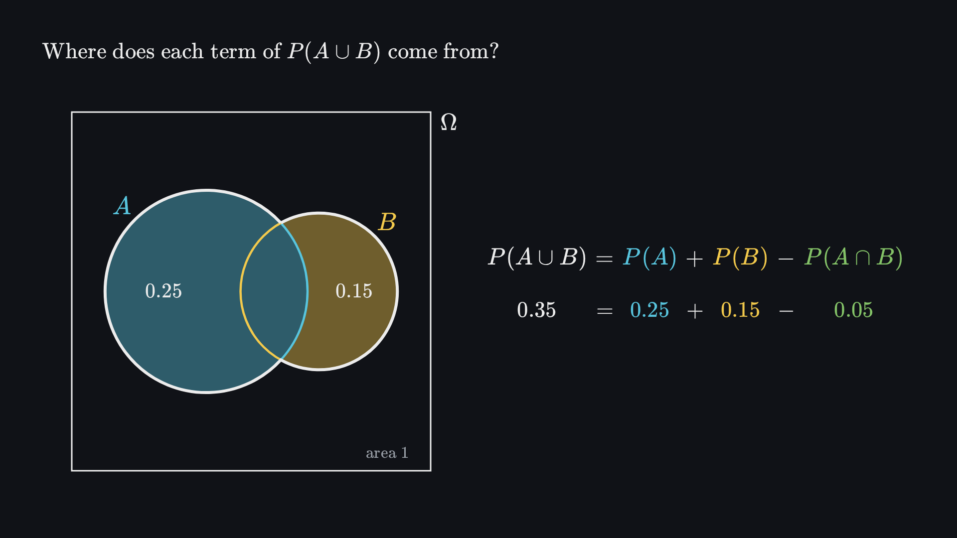

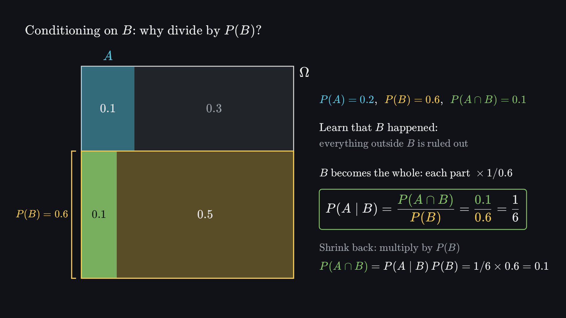

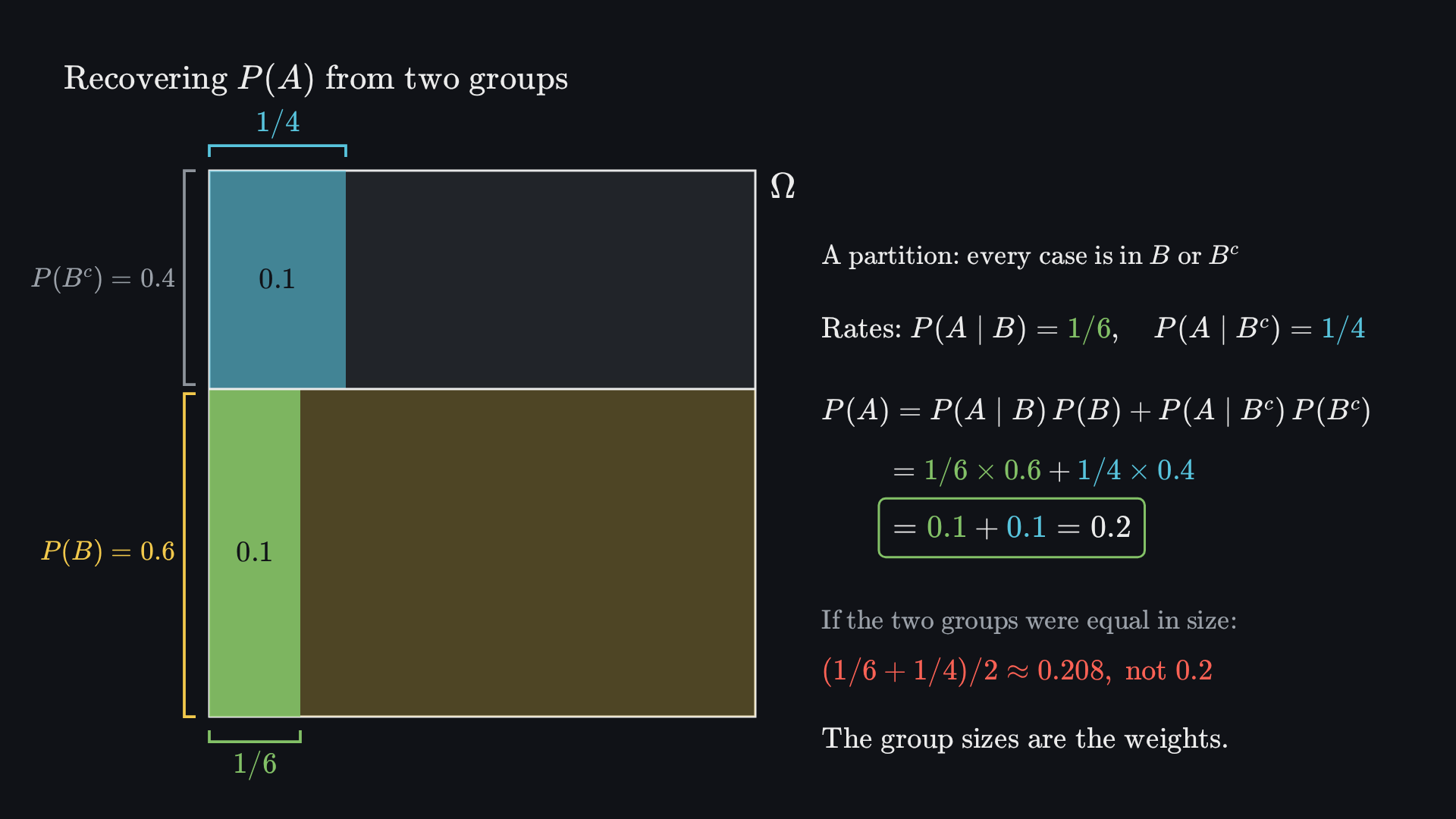
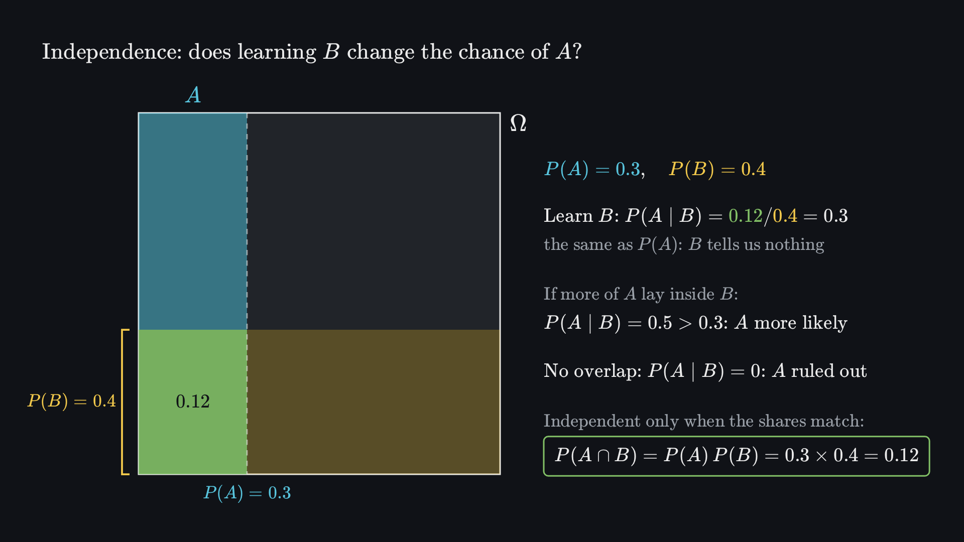

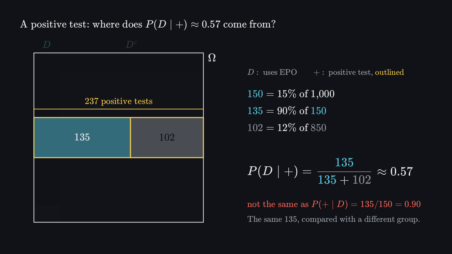
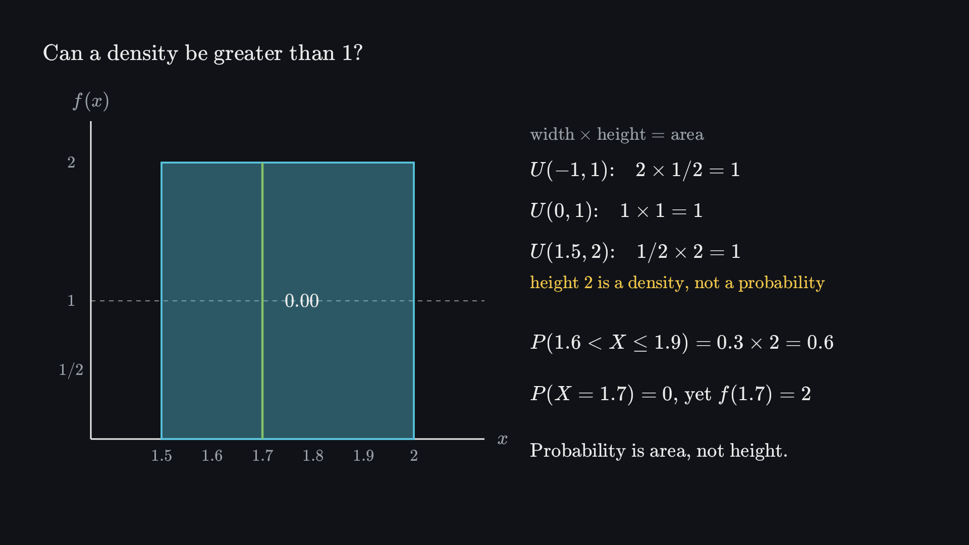
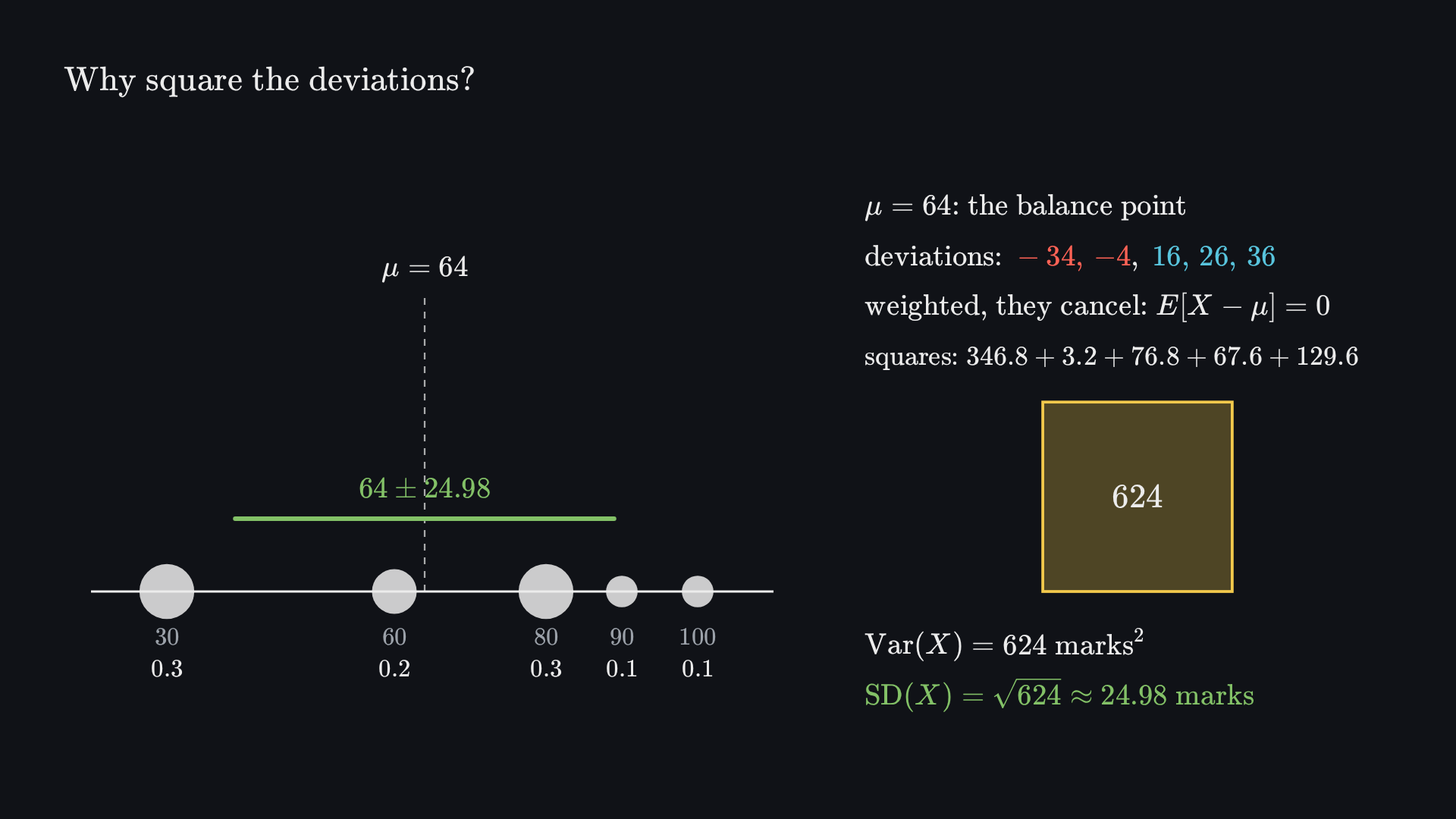
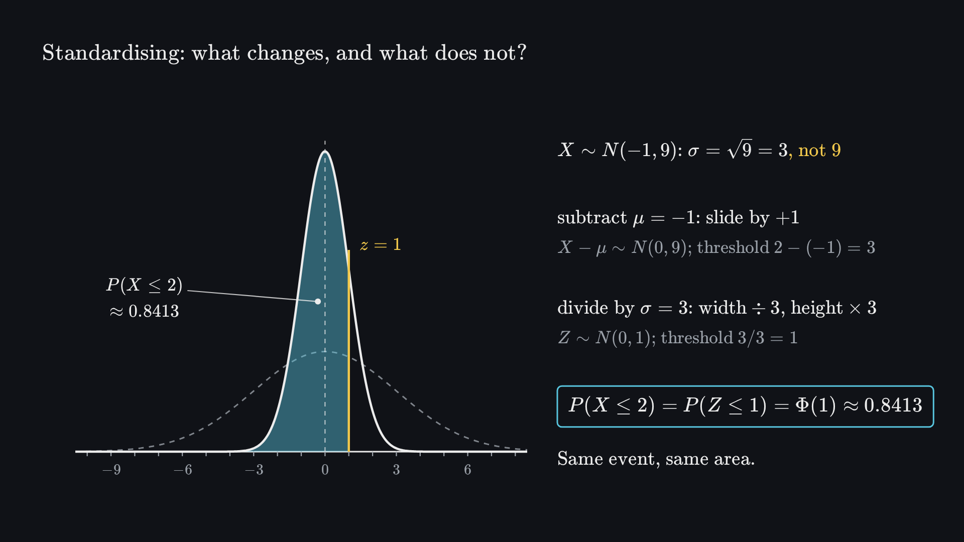
![Final frame: three number lines. On the rows X = 1 and X = 0, balance points mark the group means 72.5 (marks 60, 60, 80, 90) and 58.33 (marks 30, 30, 30, 80, 80, 100). On the bottom line, a stack of 6 dots at 58.33 (weight 0.6) and a stack of 4 dots at 72.5 (weight 0.4) balance at the class mean 64. Beside it: E[Y | X = 1] = 290/4 = 72.5 with P(X = 1) = 0.4; E[Y | X = 0] = 350/6 ≈ 58.33 with P(X = 0) = 0.6; E[Y] = 640/10 = 64; E[E[Y | X]] = 0.4(72.5) + 0.6(175/3) = 29 + 35 = 64; so E[Y] = E[E[Y | X]], not (72.5 + 58.33)/2 ≈ 65.42.](media/iterated-expectation-end.png?v=d2c628f8e2)
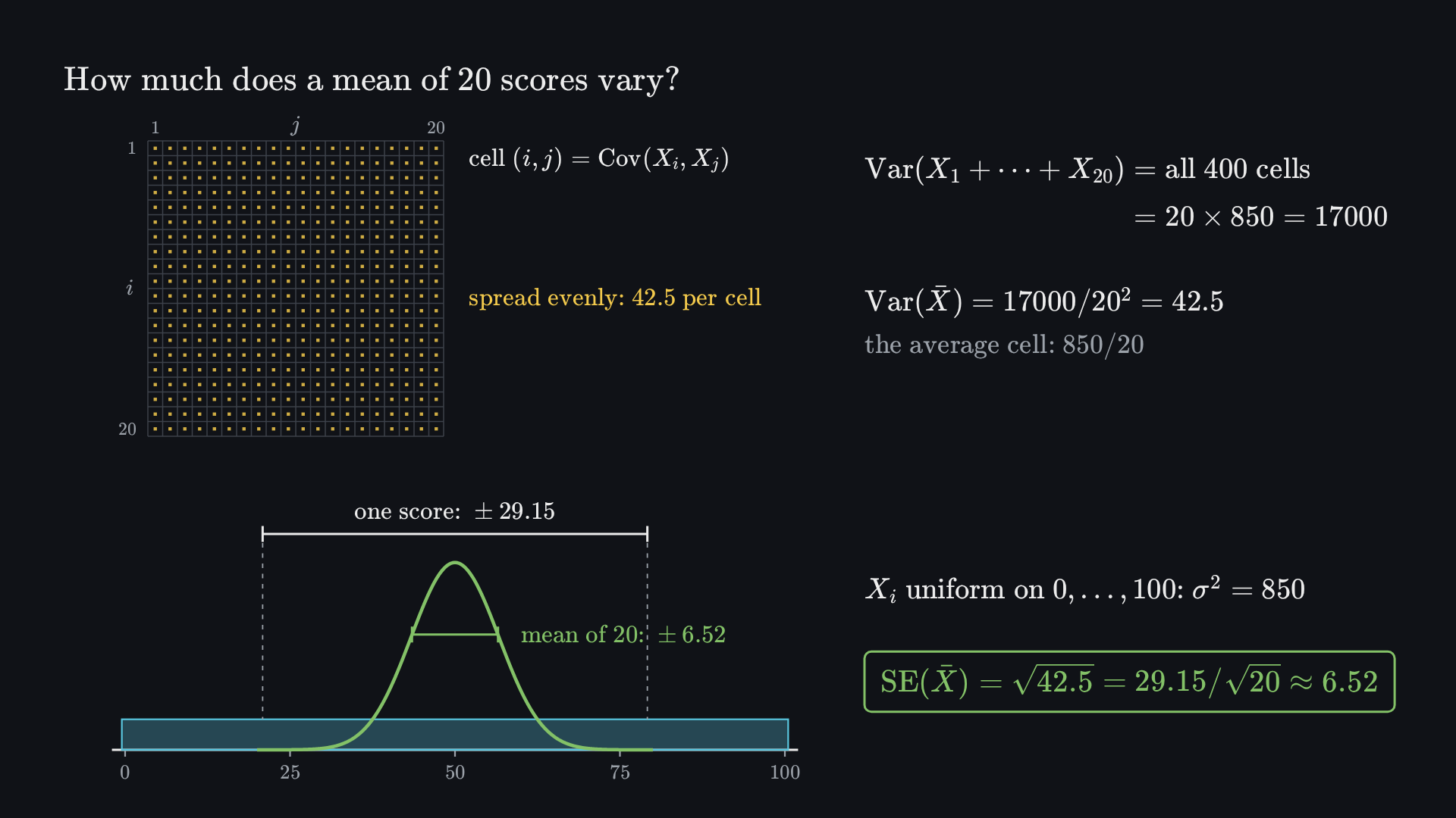
![Final frame: the sampling distribution of the mean, N(0, 1/5), with its central 95% between −0.877 and 0.877 shaded and its two 2.5% tails in red; dashed lines continue the band’s edges down the page, and a fixed dashed line marks μ = 0. Below, 40 simulated intervals x̄ ± 0.877: those whose mean lies inside the band cross the μ line (green); 3 whose mean lies outside miss it (red). Beside it: n = 5 from N(0, 1), X̄ ~ N(0, 1/5); 1.96/√5 ≈ 0.877, so P(|X̄ − μ| ≤ 0.877) = 0.95; each sample gives the interval x̄ ± 0.877; 1.00 ± 0.877 = [0.123, 1.877] misses 0; a miss happens exactly when x̄ lands outside the 95% band; this run: 37 of 40 contain 0; 95% describes the procedure over many samples, and one computed interval either contains μ or not.](media/coverage-end.png?v=3306c2f419)
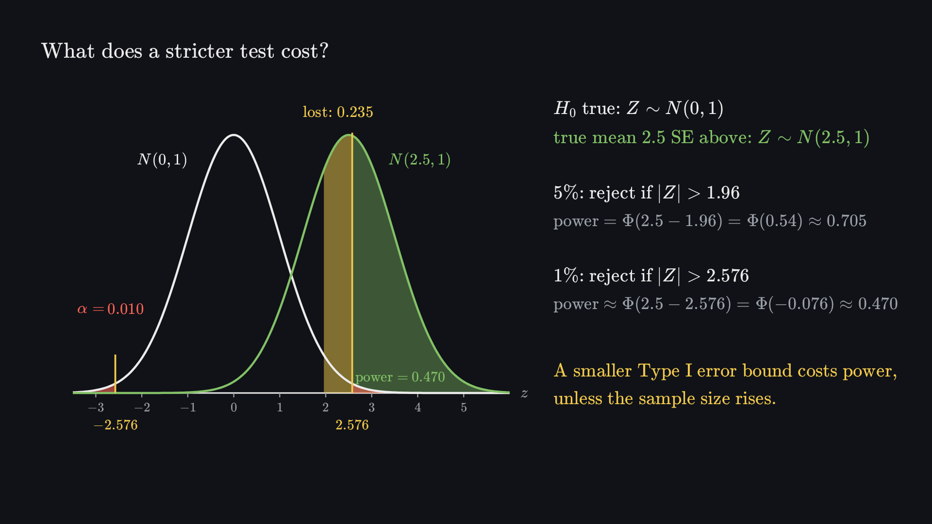
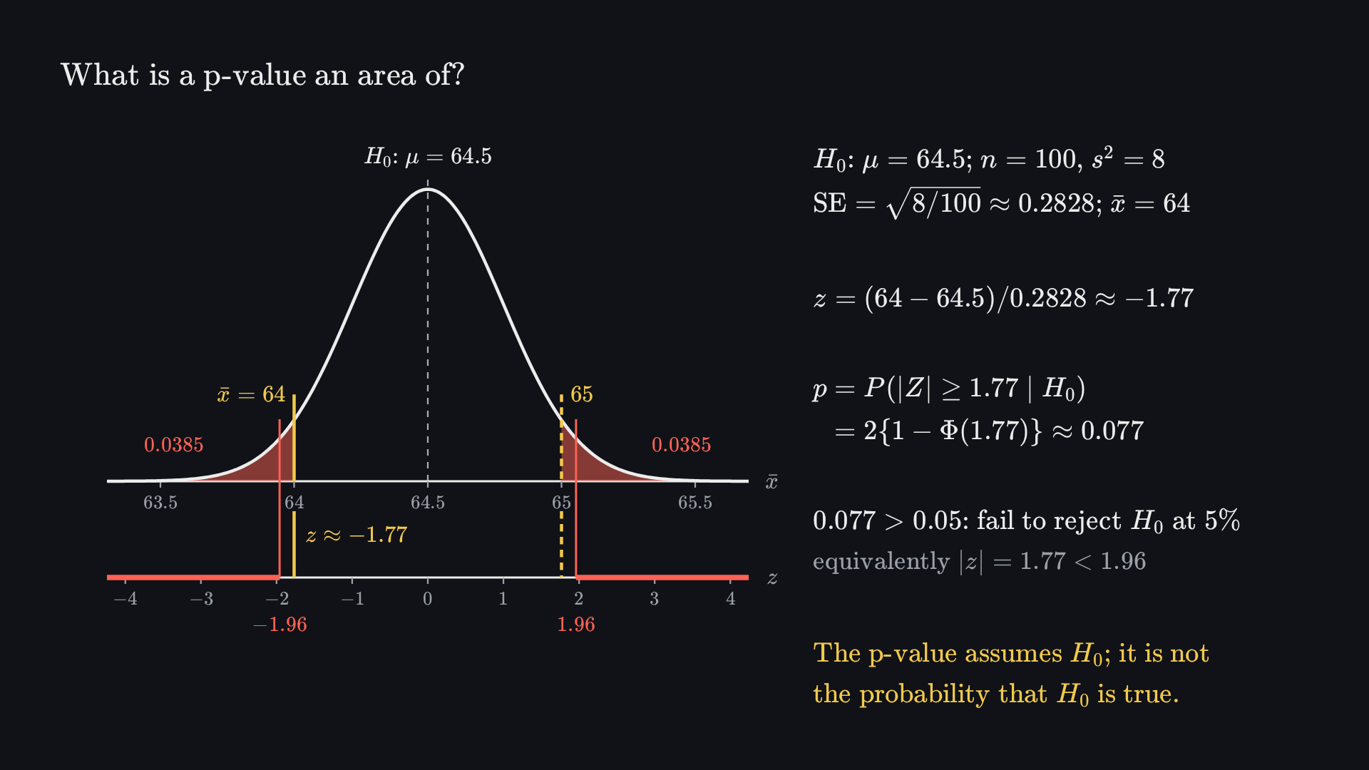
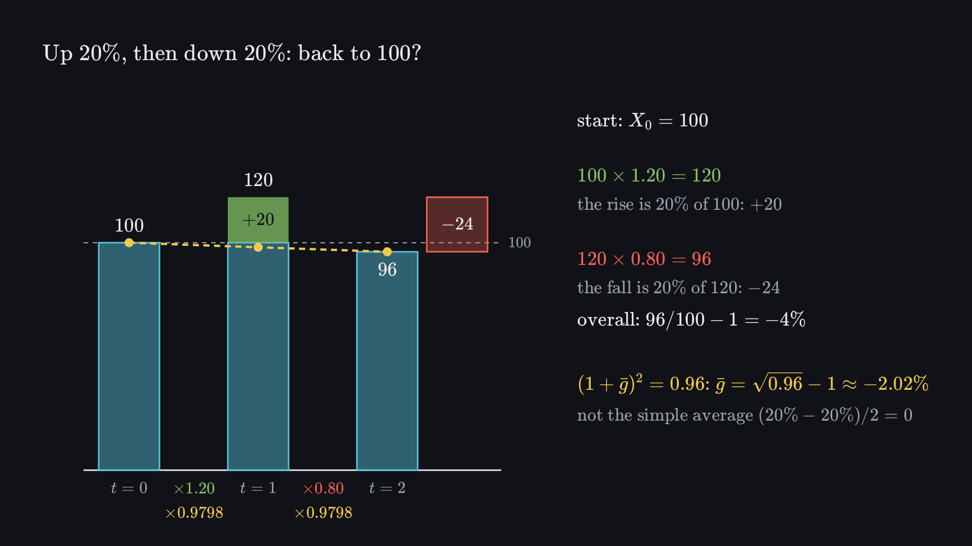
![Final frame: a time plot with the mean μ = 10 dashed. An illustrative past path rises to X_t = 15. From there the forecast centre falls towards 10 (14, 13.2, 12.56, …), inside a shaded 95% band that widens and then levels off between dashed limits 10 ± 3.27; two steps ahead, a yellow bracket marks [10.69, 15.71]. Three simulated green paths continue from 15, and one first rises to about 15.6. Beside it: μ = 10, φ = 0.8, σ² = 1, X_t = 15; X̂_{t+h|t} = 10 + 0.8^h(15 − 10) = 14, 13.2, 12.56, … → 10; V₂ = 1 + 0.8² = 1.64; 13.2 ± 1.96√1.64 = [10.69, 15.71]; V_h → 1/(1 − 0.8²) ≈ 2.78, so the band levels off. The expected deviation shrinks; a realised value can still rise.](media/ar-forecast-end.png?v=b9fd44690f)
![Final frame: a scatter of 300 simulated people, first score S₁ against retest score S₂, with a dashed no-change line S₂ = S₁ and a green conditional-mean line of slope 0.6. A strip of first scores near 30 is highlighted; a sideways yellow curve shows their retest distribution N(38, 8²), with an arrow up from 30 to 38 marked +8. A strip near 80 shows the curve N(68, 8²), with an arrow down from 80 to 68 marked −12. Beside it: S₁ = 50 + A + U₁ and S₂ = 50 + A + U₂, Var(A) = 60 persists and Var(U_i) = 40 is fresh; E[S₂ | S₁ = 30] = 50 + 0.6(30 − 50) = 38, +8 with no programme at all; E[S₂ | S₁ = 80] = 50 + 0.6(80 − 50) = 68; r = 60/(60 + 40) = 0.6, slope 0.6, not 1. Extreme first scores carry unusual noise; the retest draws fresh noise. A before–after gain is not a programme effect.](media/regression-mean-end.png?v=1be84b1182)