A probability question needs a precise description of what would make its answer “yes”. A die roll produces one face, but “the result is even” is true for three faces. A bulb has one realised lifetime, but “it survives at least ten hours” is true for many possible lifetimes. Representing each question as a set lets us calculate with these different kinds of uncertainty using the same rules.
Definition. An outcome is one possible result. The sample spaceΩ is the set of all possible outcomes considered by the model. An eventA is a subset of Ω: the outcomes for which a specified statement is true.
Write ω∈Ω for an individual outcome and A⊆Ω for an event. If the realised outcome belongs to A, the event occurs. Membership is a yes-or-no statement about that outcome. The probability P(A) describes uncertainty before learning the outcome. Different events may occur in the same experiment: one die result can be both even and prime.
Definition. The event spaceF is the collection of events to which probabilities are assigned. A probability functionP assigns each event A∈F a number P(A) between 0 and 1, consistently with the axioms in Section 1.1.4.
The three objects (Ω,F,P) form a probability model. They specify what could happen, which events are allowed, and how much probability each event receives. The letter P names a function; the parentheses in P(A) say which event is its input. A fair die and a loaded die can have the same possible outcomes and the same events, but different probability functions.
The unit scale makes comparisons consistent: probability 0.25 represents one quarter of the whole model's mass, or 25%. It does not promise that exactly one quarter of every short sequence of experiments will realise the event. A probability assignment and an observed frequency are different objects.
Formal precision: allowed events
An event space is a sigma-algebra: it contains Ω, complements of its events, and countable unions of its events. “Closed under” these operations means their results remain in the collection. This ensures that combining allowed questions produces another allowed question.
In our finite models we allow every subset, including the empty set and the whole space. An event is measurable here when it belongs to the chosen event space, so the model assigns it a probability. In continuous models the usual measurable collection contains intervals and their countable combinations; it need not contain every imaginable subset. This technical restriction does not prevent us from asking the lifetime questions considered here.
Before calculating: Name the experiment, describe one outcome, and identify all outcomes that make the event true. Then ask what probability weights the model supplies.
1.1.2 Three sample spaces
A die: fairness supplies the probability weights
For one roll of a six-sided die, consider three questions: is the result six, even, or prime?
ΩAC={1,2,3,4,5,6},={6},B={2,4,6},={2,3,5}.
Here A means “six”, B means “even”, and C means “prime”. Braces collect the outcomes belonging to a set. The number 2 is an outcome; {2} is the event containing that outcome. Rolling it makes both B and C occur.
A fair die assigns probability 1/6 to each face. Adding the three distinct even-face probabilities gives
P(B)=61+61+61=∣Ω∣∣B∣=63=21.
The counting fraction works because the outcomes are equally likely. Each selected face contributes the same weight. For any finite model, the general calculation is to add the weights of the distinct outcomes in the event; the fair model makes those weights equal.
For a concrete hypothetical loaded die, give each of faces 1 to 5 probability 0.1, and give face 6 probability 0.5. These nonnegative weights sum to 1. The event B is still {2,4,6}, but now
P(B)=0.1+0.1+0.5=0.7.
The prime event C still has three faces, yet its probability is 0.1+0.1+0.1=0.3. Equal numbers of outcomes need not mean equal probability. Loading changes the weights, not whether a face is even or prime.
Fair die, event E={2,4,6}: P(E)=3/6=1/2. For even or prime the selected set is {2,3,4,5,6}, with probability 5/6; for even and prime it is {2}, with probability 1/6.
First select the faces belonging to the event. Then count them under the fair-die assumption. Event labels inside the interaction refer to its current selections.
A coin: an event space is a set of sets
Model one toss as having two recorded outcomes: H for heads and T for tails. This model excludes other recorded results. Then
ΩF={H,T},={∅,{H},{T},{H,T}}.
The four events are neither outcome, heads, tails, and either outcome. The symbol ∅, read “the empty set”, denotes an impossible event; the whole sample space is a certain event. Notice the two levels of braces: {H} contains an outcome, while F contains events. Each of the two outcomes can be included or excluded, giving 22=4 events.
Enumerating events requires no fairness assumption. We could assign heads any probability p between 0 and 1, then assign tails 1−p. Here p, read “pee”, is a model parameter. The probability of heads becomes 1/2 only when fairness supplies that value.
A bulb: intervals replace lists of outcomes
To ask whether a bulb fails early or lasts through a required period, model its finite lifetime in hours by a nonnegative real number t, with Ω=[0,∞). For example, consider
{t:0≤t≤100},{t:t≥10},{t:30≤t≤40}.
These mean at most 100 hours, at least 10 hours, and between 30 and 40 hours. The inequalities determine membership: a realised lifetime of 35 hours belongs to all three events; a lifetime of 150 hours belongs only to the second.
The sample space contains infinitely many lifetimes. A finite counting fraction cannot supply an interval's probability, and no uniform probability exists over this entire unbounded half-line. Nor does a longer interval automatically have more probability than a shorter one elsewhere. A lifetime distribution supplies the weights; its construction is developed in the next topic.
An event can be an interval
Each thick segment is the set of lifetimes satisfying the statement. Filled endpoints are included. The arrow in the middle row continues beyond every finite lifetime. A segment’s length alone does not give its probability: that requires a lifetime distribution.
Separate two questions: Is a given lifetime in the interval? How much probability does the model assign to that interval? The first follows from the inequalities; the second needs a distribution.
1.1.3 “Not”, “and” and “or”
Set operations let us build a new question from existing questions. They first determine which outcomes belong to the event; probabilities are assigned afterwards.
Statement
Event
Membership requirement
Not A
Ac
Inside Ω, outside A.
A and B
A∩B
Inside both sets.
A or B
A∪B
Inside at least one, including both.
A, but not B
A∖B
Inside A, outside B.
Probability uses inclusive “or”. An outcome in both events belongs to their union once. Events are disjoint, or mutually exclusive, when A∩B=∅; then they cannot occur together.
For the die, B∩C={2} and B∪C={2,3,4,5,6}. The complement of even is Bc={1,3,5}. These statements concern membership and remain true for a loaded die.
A picture of “and”, “or” and “not”
The left oval is the even event B; the right oval is the prime event C. Only 2 lies in both. The union contains every labelled outcome except 1. The complement of even contains 1,3,5. Oval areas do not encode probabilities: the labelled outcomes determine membership.
Before adding probabilities: List the distinct included outcomes. Does any outcome satisfy both statements? “Even or prime” includes the face 2 once, although it answers both questions.
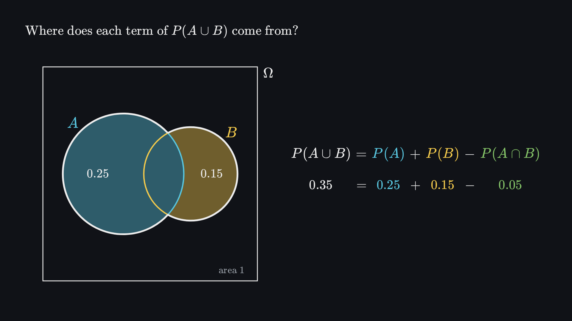
For a separate pair of events, suppose P(A)=0.25, P(B)=0.15, and P(A∩B)=0.05. Their four disjoint regions have probabilities 0.20 for A only, 0.05 for both, 0.10 for B only, and 0.65 for neither. Their total is 1. We obtain these values by keeping the overlap in its own region, then subtracting it from each marginal; Section 1.1.5 justifies that accounting.
Region
A only
Both
B only
Neither
Mass
0.20
0.05
0.10
0.65
The union comprises the first three regions: 0.20+0.05+0.10=0.35. Not A comprises the last two: 0.10+0.65=0.75.
A quantitative diagram divides probability mass into non-overlapping regions. Select “and”, “or” or “not” and identify which regions the statement includes before reading the answer.
In a quantitative diagram, area or width is deliberately scaled to probability. A unit square can represent the whole model, with total probability 1; a region occupying one quarter then represents probability 0.25. An ordinary Venn diagram need only represent membership and overlap: its drawn areas need not equal probabilities. Read the diagram’s scale before interpreting its geometry.
1.1.4 The axioms of probability
The axioms impose consistency on probability assignments. They prohibit negative mass, fix the total, and specify how distinct parts combine. They do not choose the weights of a particular die or lifetime model.
Axiom 1 — nonnegativity. For every allowed event, P(A)≥0.
Axiom 2 — normalisation.P(Ω)=1.
Axiom 3 — countable additivity. For pairwise disjoint events A1,A2,…,
P(i=1⋃∞Ai)=i=1∑∞P(Ai).
“Pairwise disjoint” means Ai∩Aj=∅ whenever i=j. The subscript labels the events; it is not part of their probability. For a finite collection, the same rule uses a finite union and sum. Distinct regions may be added because no outcome's probability mass is counted twice.
For example, two disjoint events with probabilities 0.2 and 0.1 have union probability 0.3. Disjoint events with masses 0.1 and 0.01 similarly have union probability 0.11. These calculations use disjointness, which prevents double counting; they require no equal-outcome assumption.
One immediate consequence is P(∅)=0. The disjoint union Ω∪∅ is still Ω. Additivity therefore gives P(Ω)=P(Ω)+P(∅); subtracting P(Ω)=1 leaves zero.
The converse needs care: an event with probability zero need not be the empty set. Continuous models can assign zero probability to a single exact value. The empty set is logically impossible; a zero-probability event is a statement about the model's mass assignment.
We now have a consistent way to add disjoint pieces. The next step is to decompose more complicated events into such pieces, then use the same axiom to derive useful rules.
1.1.5 Four rules, derived from the axioms
Complement rule
Goal: Express the probability outside A using P(A).
Proposition.P(Ac)=1−P(A).
Before playing, decide which axiom makes the total 1 and which one lets you add. The animation then derives the rule in four steps.The animation’s final frame. Its numbered steps describe how the picture is built.
A takes 0.25 of the area. Everything else in Ω is Ac.
Together they make Ω, so P(A∪Ac)=P(Ω)=1 by Axiom 2.
They do not overlap, so P(A∪Ac)=P(A)+P(Ac) by Axiom 3.
Equate the two expressions: P(A)+P(Ac)=1.
Rearrange: P(Ac)=1−P(A)=1−0.25=0.75.
Set identity. Every outcome is in A or outside it, so A∪Ac=Ω and A∩Ac=∅.
Disjoint additivity and normalisation.P(A)+P(Ac)=P(Ω)=1.
Rearrangement. Subtract P(A) from both sides.
If an event has probability 0.25, its complement has probability 1−0.25=0.75. Also, nonnegativity of the complement gives P(A)≤1. Together with Axiom 1, this proves the familiar bound 0≤P(A)≤1.
The rule is useful when “not” is easier to describe than the desired event. For a bulb, “lasts more than 100 hours” is the complement of “lasts at most 100 hours.” The endpoint belongs to the latter event, so the two events are disjoint and exhaustive.
Union rule: remove the duplicated overlap
Proposition.P(A∪B)=P(A)+P(B)−P(A∩B).
Adding the two marginal probabilities counts their intersection twice. Here “marginal” means the probability of each event considered separately, regardless of whether the other occurs. The derivation makes the required subtraction precise.
Play to see each term of P(A∪B)=P(A)+P(B)−P(A∩B) come from the picture. The areas are drawn to scale, so every probability is an area.The animation’s final frame. Its numbered steps describe how the picture is built.
Ω has area 1. The events A and B are drawn to scale.
Paint A:P(A)=0.25 includes the overlap.
Paint B: the overlap is now painted twice, so 0.25+0.15=0.40 is too large.
Lift off the second copy of the overlap. It becomes the subtracted term, −P(A∩B)=−0.05.
Outline the union: each point is counted once, so P(A∪B)=0.35.
Disjoint decomposition of A.A=(A∖B)∪(A∩B). Additivity gives P(A)=P(A∖B)+P(A∩B).
Rearrangement.P(A∖B)=P(A)−P(A∩B).
Disjoint decomposition of the union.A∪B=(A∖B)∪B. These parts are disjoint, so additivity gives P(A∪B)=P(A∖B)+P(B).
Substitution. Insert Step 2 into Step 3 to obtain the proposition.
With the probabilities from Section 1.1.3, the rule gives 0.25+0.15−0.05=0.35. Adding the three included regions, 0.20+0.05+0.10, gives the same answer. The overlap is subtracted once because the desired union must still include it once.
Union bound
Proposition.P(A∪B)≤P(A)+P(B).
Union rule: the union is the sum minus P(A∩B). Nonnegativity: this subtracted quantity is at least zero. Subtraction cannot increase the sum, which proves the bound. Equality holds when the overlap has probability zero; disjoint events guarantee that condition. The bound may exceed 1, so min{1,P(A)+P(B)} is a tighter upper bound when necessary. Here min means “the smaller of”.
Logical consequence, or monotonicity
Proposition. If B⊆A, then P(B)≤P(A).
Set inclusion. If B occurs, A must occur: every outcome of B is in A.
Disjoint decomposition and additivity.A=B∪(A∖B), hence P(A)=P(B)+P(A∖B).
Nonnegativity.P(A∖B)≥0, so P(A)≥P(B).
Adding a requirement restricts an event to a subset and cannot increase its probability. For the fair die, “six” implies “even”. In Section 1.1.2 these were A={6} and B={2,4,6}, so that inclusion gives P(A)=1/6≤P(B)=1/2. The letters do not determine which set is larger; identify the actual inclusion before applying the rule.
The same relationship holds for the hypothetical loaded die: 0.5≤0.7. Its numerical probabilities change, but the logical implication does not. Set relationships constrain every valid probability assignment.
1.1.6 Exercises with worked reasoning
For each question, identify the outcomes first. State the probability assumption, choose a rule, and explain why its conditions hold. Distinguish an exact answer from a bound: knowing that an event lies inside another can restrict its probability without determining it.
Exercise 1. For the fair die with B={2,4,6}, C={2,3,5}, find the probabilities of “even and prime”, “even or prime”, and “not even”. Explain why adding P(B)+P(C) alone is incorrect.
Solution
Intersection and fairness. Only 2 belongs to both sets: P(B∩C)=1/6.
Union rule.P(B∪C)=3/6+3/6−1/6=5/6. The naive sum counts the face 2 twice.
Complement rule.P(Bc)=1−3/6=1/2. Its outcomes are {1,3,5}.
Exercise 2. Given P(A)=0.25, P(B)=0.15, P(A∩B)=0.05, recover all four disjoint regions. Find the probability of neither event and check the union bound.
Solution
Disjoint decomposition.A-only has mass 0.25−0.05=0.20; B-only has mass 0.15−0.05=0.10. Both has mass 0.05.
Additivity. The union has mass 0.20+0.10+0.05=0.35.
Complement rule. Neither is (A∪B)c, with mass 1−0.35=0.65. All four masses are nonnegative and sum to 1.
Union bound.0.35≤0.25+0.15=0.40. The difference is exactly the overlap 0.05.
Exercise 3. Suppose a hypothetical bulb-lifetime model assigns probability 0.8 to lasting at most 100 hours. Could the probability of lasting between 30 and 40 hours be 0.9? Does the supplied probability determine the exact answer?
Solution
Inclusion.[30,40]⊆[0,100].
Monotonicity and nonnegativity.0≤P(30≤t≤40)≤0.8. Therefore 0.9 is inconsistent.
What remains unspecified. The model has not said how the mass within [0,100] is distributed. We have a bound, not an exact probability. A fuller lifetime distribution is required.
These rules combine probabilities within a fixed model. The next chapter considers what changes when we learn that a particular event has occurred.
1.2 Conditional probability
Information, reference groups and weighted probabilities
1.2.1Information changes the question
A probability describes uncertainty relative to the information available. Before learning anything else, we consider the whole sample space. After learning that an event occurred, we consider only possibilities consistent with that event. Conditional probability expresses this change of reference group: among the possibilities compatible with what we know, how much probability belongs to the event we are asking about?
Consider a family with two children. Use a toy model in which each child has a boy or girl outcome, each with probability 1/2. Assume the two outcomes are independent: knowing one does not change the probabilities for the other. Order the children from older to younger, writing b for boy and g for girl. These assumptions define the exercise; they are not demographic claims. The sample space is
Ω={(b,b),(b,g),(g,b),(g,g)}.
Independence gives each ordered pair probability (1/2)(1/2)=1/4. The mixed pairs are distinct: (b,g) has an older boy, while (g,b) has an older girl. Let A be “two boys” and B be “at least one boy.” Then
AB={(b,b)},={(b,b),(b,g),(g,b)}.Before playing, predict: once you know there is at least one boy, is two boys more or less likely than 1/4?The animation’s final frame. Its numbered steps describe how the picture is built.
Four equally likely families: each has probability 1/4.
Two boys is one of them: P(A)=1/4.
Learn B, that there is at least one boy: (g,g) is ruled out.
The three that remain share the whole, a third each, so P(A∣B)=(1/4)/(3/4)=1/3.
No family changed; only the group we compare with did.
Specify how the information is obtained. Choose a family at random from this model, check whether it has at least one boy, and retain it exactly when B is true. This procedure excludes (g,g) without favoring one of the three retained outcomes over another. Of the retained probability 3/4, the part belonging to two boys is 1/4. Therefore
P(A∣B)=3/41/4=31.
Before screening, the probability of two boys was 1/4; within the screened group it is 1/3. No family has changed. We have changed the group within which the fraction is calculated.
Different information procedures give different answers
If we instead learn that the older child is a boy, only (b,b) and (b,g) remain. They are equally likely, so the probability of two boys is 1/2. “The older child is a boy” and “at least one child is a boy” are different events, even though both imply that the family has a boy.
Now choose one of the two children at random, independently of the family’s outcomes, and observe that the selected child is a boy. A two-boy family always produces that observation; a mixed family produces it only half the time. Mixed families therefore receive less weight than two-boy families among observations of a boy. To count explicitly, pair each of the four family outcomes with either choice of child. There are eight equally likely family–child pairs. Four produce a boy: two from (b,b), one from (b,g), and one from (g,b). Two of those four come from a two-boy family, giving 2/4=1/2.
The statement we heard is not enough to justify a calculation if its reporting procedure is unspecified. In particular, a parent choosing which child to mention need not reproduce either procedure above. First define what was checked or observed; then identify the outcomes and weights consistent with that information.
Ordered outcome
At least one boy
Older child a boy
(b,b)
Retained
Retained
(b,g)
Retained
Retained
(g,b)
Retained
Excluded
(g,g)
Excluded
Excluded
With independent children’s outcomes and equal boy/girl probabilities, these conditioning events give probabilities of two boys 1/3 and 1/2, respectively.
Compare screening for at least one boy with knowing the older child is a boy under the same family model. Predict which outcomes remain before inspecting the answer.
1.2.2Restriction, normalization and the definition
Counting retained outcomes worked above because the relevant cases were equally likely. The general definition uses their probability weights instead. Let A be the event we want to assess and B the information on which we condition.
Definition. For events A and B, provided P(B)>0,
P(A∣B)=P(B)P(A∩B).
The numerator is not P(A): some outcomes in A may be incompatible with the information. We retain only the intersection A∩B, meaning outcomes where both events occur. The denominator is not the probability of the whole sample space: our reference group is now B. We divide the retained part of A by the probability of that entire reference group.
Why divide by the probability of the information?
Restriction. Exclude outcomes outside B. The retained part of A is A∩B, with its original probability P(A∩B).
Preserve relative weights. Apply one common multiplier c to all retained probabilities. If one retained part originally had twice the probability of another, it must still have twice the probability after conditioning.
Normalize. The entire retained group must have conditional probability one. Thus cP(B)=1, which gives c=1/P(B).
Apply the multiplier. The conditional probability of A is cP(A∩B)=P(A∩B)/P(B).
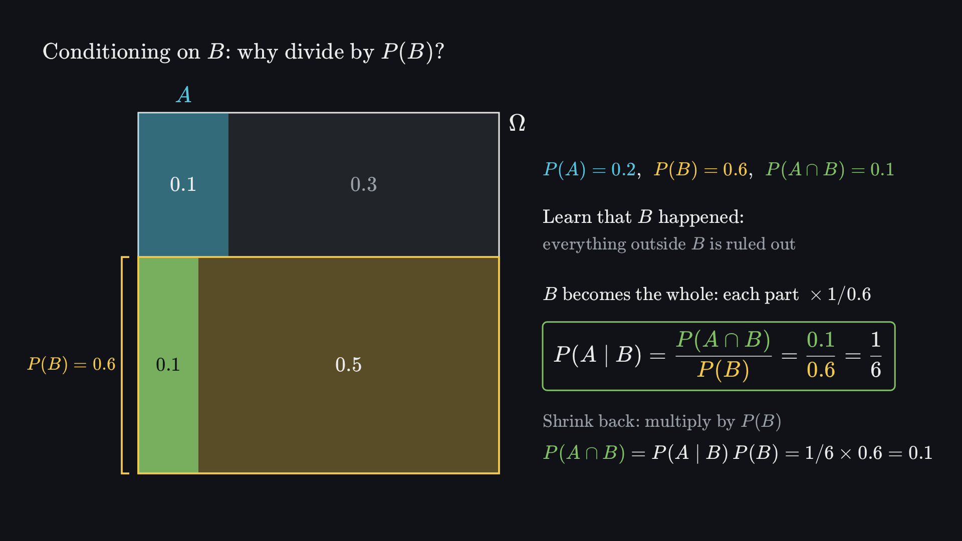
Before playing, predict: when B is stretched to fill the whole square, what share of it will the overlap fill?The animation’s final frame. Its numbered steps describe how the picture is built.
The model: P(A)=0.2,P(B)=0.6 and P(A∩B)=0.1.
Learn that B happened: everything outside B is ruled out.
B swells to fill the square. Every part of it grows by the same factor, 1/0.6, so the overlap keeps its share of B:1/6.
So P(A∣B)=P(A∩B)/P(B)=0.1/0.6=1/6, and the two parts of B still add to 1.
Shrinking back multiplies by P(B):P(A∩B)=P(A∣B)P(B)=1/6×0.6=0.1.
This process is called renormalization: restoring a total of one after restriction. For example, suppose P(A)=0.2, P(B)=0.6 and P(A∩B)=0.1. The intersection contributes probability 0.1, and the rest of B contributes 0.6−0.1=0.5. Write Ac, read “A complement,” for not A. Conditioning scales these two retained parts by 1/0.6:
P(A∣B)P(Ac∣B)=0.60.1=61,=0.60.5=65.
The rescaled parts add to one. The original probability P(B) remains 0.6; the new probability P(B∣B) is one. Conditioning creates a different probability assessment rather than overwriting the original one.
Keep the information group, then rescale it
Whole model
P(A∩B)=0.10 inside P(B)=0.60.
Within the retained group
0.10/0.60=1/6 of the new total.
In the whole-model diagram, the dashed boundary encloses B; its two lower regions have total mass 0.60. Only the lower-left piece also belongs to A. The retained-group diagram redraws the retained mass as a new whole: the event of interest occupies one sixth. Conditioning changes the reference group, not which outcomes lie in the intersection.
The product rule reverses the rescaling
If P(A∣B) describes the fraction inside B, multiplying by the size of B restores its share of the original whole:
Product rule. When P(B)>0,
P(A∩B)=P(A∣B)P(B).
Conditional definition. Begin with P(A∣B)=P(A∩B)/P(B).
Multiply both sides by the denominator. This gives the displayed product rule.
The left side is a joint probability: the probability that both events occur. It equals the probability of belonging to B, multiplied by the fraction of that group also in A. Replacing P(A∣B) with P(A) would be an additional claim that the information B leaves the probability of A unchanged. The next chapter identifies that condition as independence.
Definition or starting axiom?
The elementary approach here defines conditional probability by the ratio and derives the product rule by rearrangement. Other foundations take a multiplication relationship as a starting point for conditional probability. This distinction does not change the calculations for positive-probability conditioning events.
The probability rules continue to hold
Keep B fixed with P(B)>0. Nonnegativity and the fact that A∩B is contained in B give
0≤P(A∣B)≤1.
The reference group is certain under its own condition, while its complement is excluded:
P(B∣B)P(Bc∣B)=1,=0.
For events A1,A2,… that are mutually exclusive withinB, conditional probabilities add. “Within B” means that no outcome in B belongs to two of these events, even if they overlap outside B.
P(i⋃Ai∣B)=i∑P(Ai∣B).
The proof uses the earlier additivity rule on the disjoint intersections with B, then divides every term by the same P(B). The notation ⋃iAi means “the union of the A sub i events,” and ∑i means “sum over i”; the list may be finite or countably infinite. In particular, the complementary parts inside B satisfy
P(Ac∣B)=1−P(A∣B).Why require a positive-probability condition?
If P(B)=0, the ratio divides by zero and is undefined. An exact value in a continuous model can have probability zero without being logically impossible. Conditioning on such values requires other constructions; the elementary event ratio cannot supply the answer.
1.2.3Reversing the condition changes the denominator
“Among cases in B, how many are in A?” asks for P(A∣B). “Among cases in A, how many are in B?” asks for P(B∣A). These are different questions about the same joint event. Provided both conditioning probabilities are positive,
P(A∣B)P(B∣A)=P(B)P(A∩B),=P(A)P(A∩B).
The intersection is symmetric: “A and B” describes the same outcomes as “B and A.” The conditional calculation is not symmetric, because it divides by a different reference group. Interchanging the letters therefore does not justify keeping the same value.
Represent the preceding probabilities using a hypothetical group of 100 cases:
Four disjoint groups with the stated probability weights
Event
B
Bc
Total
A
10
10
20
Ac
50
30
80
Total
60
40
100
Before playing, predict: are P(A∣B) and P(B∣A) equal here? Both count the same 10 cases in A∩B.The animation’s final frame. Its numbered steps describe how the picture is built.
A hypothetical group of 100 cases: 20 in A,60 in B and 10 in both.
Among the 60 cases in B,10 are in A:P(A∣B)=10/60=1/6.
Gather the 20 cases in A: half of them, 10, are in B, so P(B∣A)=10/20=1/2.
The same 10 cases, compared with different groups, give different answers.
Conditioning on B selects the column containing 60 cases. Its 10 cases in A give P(A∣B)=10/60=1/6. Conditioning on A selects the row containing 20 cases. Its 10 cases in B give P(B∣A)=10/20=1/2. The 10 cases in both events have not changed; the group used to interpret them has.
A verbal example makes the distinction clear. Suppose most students in a hypothetical population are Democrats. That need not mean that most Democrats in that population are students: the Democrat group may be much larger and include many nonstudents. One fraction uses the student total; the other uses the Democrat total. A larger denominator makes the fraction smaller for the same overlap, but group sizes and overlap are both needed to calculate how small.
Reverse conditionals can coincide in particular models. For example, if the two reference groups have the same positive probability, the equal numerators and denominators give equal answers. Equality in one example is not a general rule. Bayes’ rule in the next chapter connects the two directions while accounting for their different denominators.
1.2.4Recovering an overall probability from groups
Conditioning isolates a group. Often we need the reverse task: combine the probabilities within several groups to recover a probability for the whole population. This requires knowing both each group’s internal rate and its share of the population.
A partition divides the sample space into groups that are exhaustive and mutually exclusive. Exhaustive means every possible outcome belongs to a group; mutually exclusive means no outcome belongs to more than one. For two groups B1 and B2,
B1∪B2=Ω,B1∩B2=∅.
Law of total probability. For this partition, provided both group probabilities are positive,
P(A)=P(A∣B1)P(B1)+P(A∣B2)P(B2).
The event A can occur through either group. First calculate the share of the whole population that belongs to a group and satisfies A; then add those disjoint contributions.
Exhaustiveness. Every outcome in A belongs to a group, so A=(A∩B1)∪(A∩B2).
Disjointness and additivity. These two pieces do not overlap, so P(A)=P(A∩B1)+P(A∩B2).
Product rule. Substitute P(A∩Bi)=P(A∣Bi)P(Bi) for each group.
Break the target event into disjoint pieces
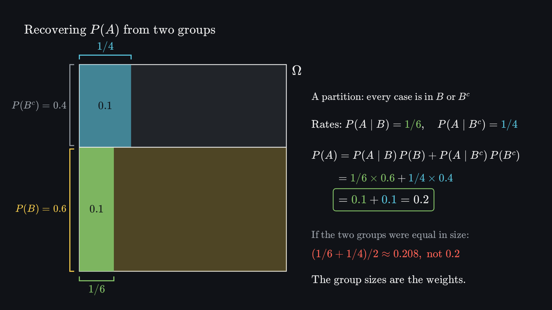
The three columns form a partition: every outcome belongs to exactly one group. The hatched event A is the union of the separate pieces A∩B1, A∩B2 and A∩B3. To recover each piece’s probability, multiply its within-group rate by the group’s probability; then add. This is a membership sketch, so drawn sizes are not assigned probabilities.Before playing, predict: is P(A) the plain average of the two group rates, 1/6 and 1/4?The animation’s final frame. Its numbered steps describe how the picture is built.
Split Ω into two groups, B and Bc, of sizes 0.6 and 0.4: every case is in exactly one.
Inside each group A has its own rate: P(A∣B)=1/6 and P(A∣Bc)=1/4.
Each rate times its group size is an area: 1/6×0.6+1/4×0.4=0.1+0.1=0.2.
Averaging the two rates would treat the groups as equal and give about 0.208. The group sizes are the weights.
Why the group probabilities are weights
The rate P(A∣Bi) is measured within group Bi, where that group is treated as the whole. Multiplying by P(Bi) converts it into a share of the original population. For an exhaustive, disjoint partition, these weights add to one. A large group contributes more than a small group with the same internal rate; simply averaging the rates would implicitly assign equal population shares.
Return to the table above. The groups B and Bc contain respectively 60% and 40% of cases. The probability of A within B is 10/60=1/6; within Bc, it is 10/40=1/4. Weight these rates by the corresponding group probabilities:
P(A)=61(0.6)+41(0.4)=0.1+0.1=0.2.
This recovers the original 20 cases in A out of 100. The two contributions are equal even though the group sizes differ: the smaller group has the higher internal rate. If the groups overlapped, adding their contributions would count some outcomes twice. If they omitted possibilities, the result would leave out some probability.
More than two groups and zero-weight groups
For a finite partition B1,…,Bk, where k is the number of groups, the same argument gives
P(A)=i=1∑kP(A∩Bi)=i=1∑kP(A∣Bi)P(Bi).
Read ∑i=1k as “sum from i equals one to k.” The joint-probability sum is valid even for a group with probability zero. The conditional form requires positive group probabilities: omit zero-weight groups before forming those ratios, rather than multiplying an undefined conditional probability by zero.
Total probability accounts for every route to an event. That will make it useful in Bayes’ rule: before asking which group an observed event came from, we must calculate how often the event occurs across all groups.
1.2.5Exercises with worked solutions
Identify the conditioning group or partition before calculating. Try each problem before opening its solution.
1. Equal answers in opposite directions
For a fair die, let A={4,5,6} and B={2,4,6}. Calculate both P(A∣B) and P(B∣A). Why do they coincide?
Solution
Intersection.A∩B={4,6}. Each face has probability 1/6, so P(A∩B)=2/6.
Conditioning groups. Both events contain three faces, giving P(A)=P(B)=3/6.
Conditional definition. Both ratios are (2/6)/(3/6)=2/3.
The equal answers follow from equal reference-group probabilities, not from a general symmetry of conditional probability.
2. Reconstruct the joint probability first
For events A and B, suppose P(A∣B)=0.8, P(B)=0.25 and P(A)=0.5. Find P(A∩B) and P(B∣A).
Solution
Product rule.P(A∩B)=0.8×0.25=0.2.
Reverse conditional. The requested reference group is A, so P(B∣A)=0.2/0.5=0.4.
Check. The joint probability is no greater than either group probability, and the conditional answer lies between zero and one.
The given 0.8 is the fraction of B cases that belong to A. The requested 0.4 is the fraction of A cases that belong to B.
3. Weight group rates
A hypothetical workshop produces 40% of its items on line B1 and 60% on line B2. Every item comes from exactly one of these lines. Defect probabilities within the two lines are respectively 0.05 and 0.10. One item is selected uniformly from all production. Find the probability that it is defective.
Solution
Define the event and groups. Let A mean defective. The two production lines form an exhaustive, disjoint partition.
Total probability.P(A)=0.05(0.4)+0.10(0.6)=0.02+0.06=0.08.
Frequency check. In 1000 hypothetical items, expect 20 defects among 400 first-line items and 60 among 600 second-line items: 80/1000=0.08.
The unweighted mean (0.05+0.10)/2=0.075 would incorrectly give the two lines equal population shares. The weighted result lies between the two internal defect rates, as a useful check.
1.3 Independence and Bayes’ rule
Relationships between events and reasoning from evidence
1.3.1 Independence: information that leaves a probability unchanged
Conditional probability lets us ask whether information changes our assessment. Independence is the particular case in which it does not. It concerns a specified pair of events under a specified probability model. To establish it, compare the probabilities before and after conditioning, rather than relying on whether the events look unrelated.
Definition. Events A and B are independent if P(A∩B)=P(A)P(B). The joint probability equals the product of the two marginal probabilities.
“Marginal” means that the probability is taken without conditioning on the other event. When P(B)>0, independence is equivalent to P(A∣B)=P(A): the proportion of A within B equals the proportion of A in the whole sample space. This explains why independent events can overlap. What matters is the size of their overlap relative to their marginals.
Proposition. If P(B)>0, the product definition and the unchanged-conditional definition are equivalent.
Conditional definition. Start with P(A∣B)=P(A∩B)/P(B). The positivity condition permits division.
Unchanged conditional implies product. Starting instead from P(A∣B)=P(A), multiply both sides by P(B): P(A∩B)=P(A)P(B).
Symmetry. Intersection and multiplication are commutative, so the product equation also gives B⊥⊥A. If P(A)>0, dividing by P(A) gives P(B∣A)=P(B).
The product definition remains meaningful when a marginal is zero. If P(A)=0, monotonicity gives P(A∩B)=0, so A is independent of every B. The fraction P(B∣A) is then undefined in our elementary conditional-probability definition. Do not divide by zero to express the symmetry.
Independence also describes the information supplied by non-occurrence. Subtract the joint mass from the marginal: P(A∩Bc)=P(A)−P(A∩B). Under independence this becomes P(A)[1−P(B)]=P(A)P(Bc). If P(Bc)>0, division therefore gives P(A∣Bc)=P(A). Neither learning that B occurred nor learning that it did not occur changes the probability of A.
How much overlap means independence?
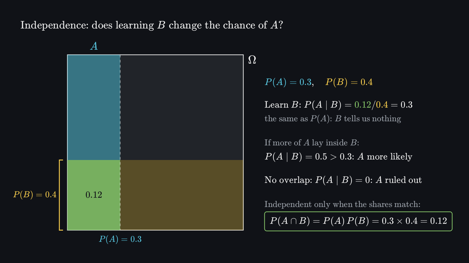
Consider P(A)=0.30, P(B)=0.40, and P(A∩B)=0.12. The independence target is 0.30(0.40)=0.12, exactly the stated overlap. Consequently, P(A∣B)=0.12/0.40=0.30, and P(B∣A)=0.12/0.30=0.40. The four disjoint region masses are 0.12 for both, 0.18 for A only, 0.28 for B only, and 0.42 for neither. They sum to one.
Before playing, predict: if A and B did not overlap at all, would they be independent?The animation’s final frame. Its numbered steps describe how the picture is built.
B is the bottom band, P(B)=0.4.A takes 0.3 of the width in both bands, so P(A)=0.3 and the overlap is 0.12.
Learn B:B swells to fill the square and A’s share of it is still 0.12/0.4=0.3. Learning B tells us nothing about A.
If more of A lay inside B, learning B would make A more likely: P(A∣B)=0.5.
If A and B did not overlap, learning B would rule A out: P(A∣B)=0. Disjoint events are dependent.
Only when the shares match is A independent of B:P(A∩B)=P(A)P(B)=0.3×0.4=0.12.
Within B, the share belonging to A is the same as in the whole sample space. If the overlap increased while the two marginals stayed fixed, knowing B would increase the probability of A. If the overlap decreased, knowing B would decrease it. The product gives the point at which those probabilities match.
P(A)
P(B)
P(A∩B)
P(A∣B)
0.30
0.40
0.12
0.30
These probabilities satisfy P(A∩B)=P(A)P(B). At zero overlap, the same positive marginals give disjoint, dependent events with P(A∣B)=0.
Keep both marginals fixed and alter the overlap. Predict whether conditioning on B increases, decreases, or leaves unchanged the probability of A before reading the result.
Disjointness answers a different question
Think first. If two positive-probability events cannot occur together, does learning that one occurred tell you anything about the other?
Disjoint events cannot occur together: A∩B=∅. If both marginals are positive, their joint probability is zero while their product is positive, so they are dependent. Knowing that B occurred rules out A: its conditional probability becomes zero. Disjointness is about which outcomes can occur together; independence is about whether information changes a probability.
The same marginals, two different relationships
Independent
P(A∣B)=0.12/0.40=0.30.
Disjoint
P(A∣B)=0/0.40=0.
Both models have P(A)=0.30 and P(B)=0.40. In the independent model, the share of A within the dashed B boundary equals its share in the whole frame. In the disjoint model, B excludes A altogether. The hatching marks B; every region’s area equals its probability.
Disjoint events with a zero marginal can be independent; the positive-probability qualification matters. Statistical dependence, in turn, does not by itself establish a causal effect.
1.3.2 Bayes’ rule: the same joint probability in two directions
Suppose we can assess how often evidence B would occur among cases where A is true. After observing B, we want the probability of A. These questions run in opposite directions. Bayes’ rule connects them by expressing the same intersection in two ways; it does not simply exchange the letters around the conditioning bar.
Bayes’ rule. When the displayed conditional probabilities are defined and P(B)>0, P(A∣B)=P(B)P(B∣A)P(A).
Before playing, predict: the overlap is 61 of B. What share of A is it?The animation’s final frame. Its numbered steps describe how the picture is built.
The model of chapter 1.2: P(A)=0.2,P(B)=0.6 and P(A∩B)=0.1.
From B’s side the overlap is 1/6 of B:P(A∩B)=P(A∣B)P(B)=1/6×0.6.
From A’s side it is half of A:P(A∩B)=P(B∣A)P(A)=1/2×0.2.
Both describe the same area, so P(A∣B)P(B)=P(B∣A)P(A).
Divide by P(B): Bayes’ rule, P(A∣B)=P(B∣A)P(A)/P(B)=(1/2×0.2)/0.6=1/6.
Derivation goal. Reconstruct the probability of both A and B from the known direction, then divide by the probability of the observed evidence.
Product rule in the first direction. For P(B)>0, P(A∩B)=P(A∣B)P(B).
Product rule in the reverse direction. For P(A)>0, P(A∩B)=P(B∣A)P(A).
Equate the common joint probability. Hence P(A∣B)P(B)=P(B∣A)P(A).
Divide by the evidence probability. Division by P(B)>0 produces Bayes’ rule.
If P(A)=0, the joint probability and P(A∣B) are zero for positive-probability B, but the reverse conditional in this derivation is undefined. Use that direct argument rather than multiplying an undefined conditional by zero.
Usually the denominator is found by total probability. The alternatives A and Ac partition the sample space, so, when both have positive probability, P(B)=P(B∣A)P(A)+P(B∣Ac)P(Ac). Multiply within each route to the evidence, then add across the disjoint routes. The denominator contains every way the evidence can occur.
This denominator is a normalizing quantity. The joint masses P(A∩B) and P(Ac∩B) add to P(B). Dividing both by that same total gives updated probabilities whose sum is one. Bayes’ rule thus preserves the basic probability accounting from Chapter 1 while changing the group within which uncertainty is assessed.
1.3.3 Worked example: a positive test among cyclists
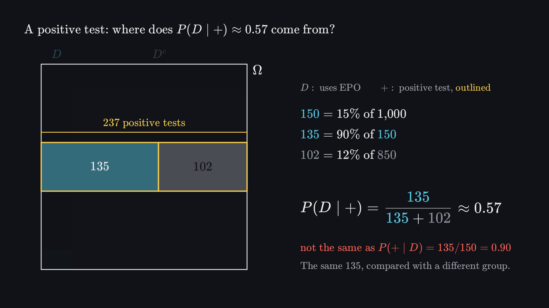
Suppose a hypothetical cycling population has 15% EPO users. A test is positive for 90% of users and 12% of non-users. These rates define the exercise’s model. Let D mean EPO use and + mean a positive test. Question: Among positive tests, what proportion are EPO users, P(D∣+)?
The known rate P(+∣D)=0.90 is the test’s sensitivity. It starts with users and asks how often they test positive. The requested updated probability, or posterior, starts with positive tests and asks how many came from users. The starting groups differ.
Follow the two routes to a positive test
Start with 1,000 hypothetical cyclists. The prior splits them into 150 EPO users and 850 non-users.
EPO use
No EPO use
Multiply along each branch: 150(0.90)=135 user positives and 850(0.12)=102 non-user positives. Add these positive leaves to find the conditioning group: 135+102=237. The posterior is the share coming through the user route, 135/237, rather than the positive-test rate on that route alone.
There are two disjoint routes to a positive test: a user tests positive, or a non-user tests positive. The numerator needs only the first route; the denominator needs both.
Total probability. The non-user positive route has mass 0.12(0.85)=0.102. Thus P(+)=0.135+0.102=0.237.
Condition on all positives.P(D∣+)=0.2370.135=7945≈0.56962≈56.96%.
Natural frequencies make the same calculation readable. In a hypothetical cohort of 1,000, the model gives 150 users and 850 non-users. Split each group according to its own test-positive rate:
Before playing, guess roughly what share of positive tests come from EPO users. The animation then traces every count in a hypothetical group of 1,000 cyclists.The animation’s final frame. Its numbered steps describe how the picture is built.
Picture a hypothetical group of 1,000 cyclists.
Prior: 15% use EPO, so 150 users and 850 non-users.
Test: 90% of the 150 users and 12% of the 850 non-users test positive, giving 135 and 102.
Keep only the positive tests: 135+102=237.
Of the 237 positive tests, 135 come from users: P(D∣+)=135/237≈0.57.
That is not the sensitivity P(+∣D)=135/150=0.90: the same 135, compared with a different group.
Expected counts in the hypothetical cohort
Status
Positive
Negative
Total
EPO use
135
15
150
No EPO use
102
748
850
Total
237
763
1,000
Assumed inputs: prior 15%, sensitivity 90%, false-positive rate 12%. The expected 135 user positives and 102 non-user positives give 135/237≈56.96%. Keeping the test fixed and changing only the prior to 1% gives 9/127.8≈7.04%.
Before reducing the prior, predict which positive-column count will fall most. Compare the posterior with sensitivity. Fractional counts are expectations under the model, not simulated observations.
At the starting assumptions, the positive column contains 135 users out of 237 expected cases. A positive test raises the model probability from 15% to about 57%. It supports EPO use while leaving substantial uncertainty about an individual’s status.
Read the user row to recover sensitivity: 135/150=0.90. Read the positive column to recover the posterior: 135/237. Both fractions have the same numerator but different denominators. Choosing a larger hypothetical cohort would multiply every table entry by the same factor and leave these fractions unchanged. The cohort is a representation of probabilities, not extra evidence about actual cyclists.
The prior proportion of users is the base rate. Although a non-user has the smaller chance of a positive result, there are many more non-users: 850 versus 150. Their false positives therefore contribute 102 of the 237 positives. Changing the base rate changes this mixture even when the test’s sensitivity and false-positive rate stay fixed.
Replace the event A by a hypothesis H and the information B by evidence E. The mathematics is unchanged; the letters make the inferential roles explicit. A hypothesis is a proposition whose truth is uncertain, and evidence is the observation on which we condition.
Bayesian update.P(H∣E)=P(E)P(E∣H)P(H).
The prior, P(H), describes uncertainty before incorporating this evidence. It may already reflect earlier information. The likelihood, P(E∣H), assesses how compatible the observation is with the hypothesis. The evidence probability, P(E), adds the contributions of all alternatives. The posterior, P(H∣E), is the updated probability after conditioning on the observation.
A likelihood is not a probability assigned to the hypothesis. To judge whether evidence supports H, compare how readily the same evidence arises under alternatives. For the positive cycling test, 0.90 exceeds 0.12, so the observation favors EPO use over non-use. The amount of updating also depends on the prior. Evidence that favors a hypothesis need not make that hypothesis certain or even more likely than its complement.
Think first. If the same evidence is equally likely under H and its complement, which hypothesis does the observation favor?
It favors neither. Provided that common likelihood is positive and both prior probabilities are positive, it cancels from the Bayes formula and the posterior equals the prior. Learning depends on how evidence distinguishes the alternatives.
Before an update, name the hypothesis, the observation, and the relevant population in words. Then ask where each input came from and which group its denominator describes. A large sample can estimate a forward rate accurately without turning it into a reverse conditional. The prior and the alternative likelihood remain necessary parts of the calculation.
The odds form makes the comparison explicit
For positive prior probabilities, positive evidence probability, and P(E∣Hc)>0, divide the two Bayes formulas. The common evidence denominator cancels:
P(Hc∣E)P(H∣E)=P(E∣Hc)P(E∣H)×P(Hc)P(H).
Posterior odds equal likelihood ratio times prior odds. In the cyclist example, the prior odds are 3/17, the likelihood ratio is 0.90/0.12=7.5, and the posterior odds are 45/34. Odds compare the two alternatives; probability compares one alternative with their total.
Later evidence can update the posterior again. Repeated test outcomes may be multiplied as separate likelihood factors only if their conditional independence is justified within each hypothesis. Shared equipment or samples may make their errors dependent. Bayes’ rule supplies the accounting relationship; it does not supply missing empirical assumptions.
1.3.5 Evidence and assumptions: the Sally Clark example
Sally Clark’s case illustrates why the assumptions behind a calculation matter. SIDS means sudden infant death syndrome. An independence argument associated with the case used a single-death frequency of roughly 1/8,500, then squared it. With that rounded value, (8,5001)2=72,250,0001, approximately one in 73 million. Squaring is justified only if the sibling deaths are independent under the relevant model. The general product rule instead requires P(S1∩S2)=P(S1)P(S2∣S1). Here Si denotes a SIDS death for child i.
The second factor asks about a family in which one such death has already occurred. Replacing it by the unconditional risk assumes that this information makes no difference. A shared familial risk can make that assumption inappropriate; the single-death frequency alone cannot settle the question.
Two distinct errors must be kept separate. First, an unsupported independence assumption can produce the wrong joint probability. Second, a small probability of evidence under an explanation does not establish that the explanation has a small probability after observing that evidence. The latter confuses P(E∣H) with P(H∣E); it is commonly called the prosecutor’s fallacy.
The Royal Statistical Society’s guide to statistical evidence explains both errors and reports the more precise historical frequency 1/8,543. A rare observation must be assessed under competing explanations, together with their prior probabilities; rarity alone supplies no posterior.
An illustrative calculation: algebra and the meaning of its inputs
Define H as both deaths being SIDS and E as both deaths being sudden and unexpected. For a toy calculation, assign h=P(H)=1/(1,300×100)=1/130,000, take P(E∣H)=1, and assign q=3/650,000 to P(E∣Hc). These assigned numbers demonstrate the algebra; their empirical interpretation must be examined separately.
Two-route denominator. Under those assumptions, P(E)=h+(1−h)q.
This is not a verified posterior for the historical case. The complement Hc contains every non-SIDS explanation, not only murder. A count per annual births does not automatically estimate the conditional probability of paired sibling deaths given a non-SIDS explanation. The quoted inputs also involve different denominators and populations. A defensible posterior would require clearly defined, comparable hypotheses and validated likelihoods; correcting one independence error does not establish those quantities.
Before calculating, specify the target question, identify the conditioning group for every rate, and justify any product of probabilities. Independence and Bayes’ rule make the reasoning explicit; conclusions inherit the limits of the model and evidence.
1.3.6 Problems and worked reasoning
Write the target probability and name its denominator before opening each solution. Use the steps to check both the calculation and the interpretation.
1. Even and prime on a fair die
Let A={2,4,6} and B={2,3,5}. Are the events independent? What is P(A∣B)?
Solution
Equal-weight counting. Each set contains three of six outcomes, so P(A)=P(B)=1/2.
Intersection. Only outcome 2 belongs to both, giving P(A∩B)=1/6.
Independence comparison. The marginal product is 1/4, which differs from 1/6. The events are dependent.
Conditioning.P(A∣B)=(1/6)/(1/2)=1/3. Knowing the outcome is prime reduces the probability of an even outcome from 1/2 to 1/3.
2. Independence in the reverse direction
Suppose P(A)=0.20, P(B)=0.50, and the events are independent. Find the joint probability and both conditionals.
Solution
Product definition.P(A∩B)=0.20(0.50)=0.10.
Condition on B.P(A∣B)=0.10/0.50=0.20.
Condition on A.P(B∣A)=0.10/0.20=0.50. Independence preserves each corresponding marginal; it does not require the two reverse conditionals to equal each other.
3. A rarer condition with the same test
Keep sensitivity 0.90 and false-positive rate 0.12, but change the cyclist prior to 1%. Find the posterior after a positive result.
Solution
User-positive route. Its mass is 0.01(0.90)=0.009.
Non-user positive route. Its mass is 0.99(0.12)=0.1188.
Total probability.P(+)=0.009+0.1188=0.1278.
Bayes.P(D∣+)=0.12780.009=715≈7.04%.
In 1,000 hypothetical cyclists, the expected positive counts are 9 users and 118.8 non-users. The test still favors use relative to the prior, but positives arise much more often from the larger non-user group.
4. Evidence that favors a hypothesis
In a separate hypothetical model, P(H)=0.25, P(E∣H)=0.60, and P(E∣Hc)=0.20. Does observing E make H certain?
Solution
Complement.P(Hc)=0.75.
Total probability.P(E)=0.60(0.25)+0.20(0.75)=0.30.
Bayes.P(H∣E)=0.15/0.30=0.50.
Interpretation. The posterior doubles the prior, so the evidence favors H. It leaves both alternatives possible. The likelihood 0.60 is neither the prior nor the posterior.
Probability formula reference
Rules and the conditions under which they apply
Definitions and formulas
These expressions describe events under a specified probability model. Positive-probability conditions are part of the conditional definitions.
Question
Expression
Not A
P(Ac)=1−P(A)
A or B
P(A∪B)=P(A)+P(B)−P(A∩B)
Union bound
P(A∪B)≤P(A)+P(B)
Logical inclusion
B⊆A⇒P(B)≤P(A)
A given B
P(A∣B)=P(A∩B)/P(B)P(B)>0.
Joint probability
P(A∩B)=P(A∣B)P(B)
Partition
P(A)=i=1∑kP(A∣Bi)P(Bi)Exhaustive, disjoint groups with positive weights.
P(H) is the prior; P(E∣H) is the likelihood; P(E) is the evidence probability; P(H∣E) is the posterior. Disjointness permits adding probabilities. Independence permits multiplying marginal probabilities. They are different conditions.