Before calculating a probability or an average, identify the unit being studied and the feature recorded for that unit. A unit might be a person, household, firm, country or examination script. A variable describes a feature whose recorded value can vary across units or across occasions. The numbers alone do not tell us what their differences mean: a category code and an income measurement require different interpretations.
For a numerical random variable, the probability experiment and its measurement are connected by X:Ω→R. Each outcome in the sample space Ω receives a numerical value. For example, selecting a script is the experiment; its mark is the value of X. Several distinct scripts can receive the same mark. Capital X names the uncertain measurement; lower-case x names one possible value.
Measurement determines which comparisons are meaningful
Type
Meaning
Example
Nominal categorical
Labels identify groups; ordering and differences need not have meaning.
Eye colour; employment coded 0 or 1.
Ordinal categorical
Order has meaning, but equal gaps or ratios are not established.
A model allows a continuum of values in an interval.
Height, handspan or a lifetime.
A binary indicator deserves special attention. Coding employed as 1 and unemployed as 0 makes its average the proportion employed. That interpretation follows from the chosen coding; an average of arbitrary eye-colour codes does not have an analogous meaning. Likewise, ordinal codes preserve ranking without establishing that the improvement from poor to fair equals the improvement from fair to good.
Measurement precision and a probability model are different choices. Wages recorded to the nearest penny are discrete records, but a continuous approximation may be useful. A rounded age is not proof that age itself is restricted to whole years. State which approximation is being used and what it is intended to describe.
2.1.2Support and several measurements
The support identifies values the model permits. A binary indicator has support {0,1}; a six-sided die has support {1,2,3,4,5,6}; a finite nonnegative lifetime can be modelled on [0,∞). Discrete supports need not be integers: a variable taking only 0.5 and 1.5 is discrete. A continuous support need not include every real number.
For a discrete distribution we usually list the values with positive probability. For a distribution with a density, support is described by the range where density can occur, including boundary points where appropriate. An observed sample range is not necessarily the population support: not observing an extreme value does not make it impossible.
A univariate measurement records one feature. A bivariate measurement records two, and a multivariate measurement records several. A household with five children whose youngest is four years old can be represented by the vector X=(5,4). The coordinates mean different things and must retain their labels. Height, weight and eye colour also form a multivariate record, even though the last coordinate is categorical.
One unit, two coordinates
The horizontal and vertical coordinates describe the same household. Axis meanings determine what the pair records.
A number-line plot can show one measurement per unit; a scatter plot can show two. Each point in a scatter plot represents a paired record from the same unit. Combining the height of one person with the weight of another would change the joint data and destroy information about their relationship. Three numerical features form points in three-dimensional space; more features remain meaningful even when they cannot be pictured directly.
2.1.3Cross-sections, time series and panels
A cross-section records units at a specified occasion. With N units, write {Xi}i=1N, where i identifies a unit. Repeated values are still separate records: three students with mark 30 are three observations, not one.
A time series records measurements in temporal order. Write {Xt}t=1T, where t identifies time and T is the number of recorded occasions. A plot of date against value helps show how the series changes. Reordering the values generally changes its meaning because its timing contains information.
There is another useful perspective: the entire path (X1,…,XT) is one realization of a T-dimensional random vector. A three-year GDP path is one point with coordinates for the three years, as well as three points in a date–value plot. Neither representation establishes independent observations. Whether components can be used as independent evidence requires assumptions about the process generating the path.
A panel follows several units over time. Write Xit: the first index identifies a unit and the second an occasion. A balanced panel observes every unit on the same complete set of occasions. An unbalanced panel has a different observed time set for some units, perhaps because units enter or leave or measurements are missing. A panel therefore combines cross-sectional and temporal variation; it does not automatically eliminate dependence within a unit.
Structure
Record
Question to ask
Cross-section
Unit i, measurement Xi
Which population and occasion?
Time series
Date t, measurement Xt
Which time order and spacing?
Panel
Unit i, date t, measurement Xit
Which unit–date combinations are observed?
2.1.4Check the interpretation before calculating
1. Codes and quantities
A survey codes poor, fair and good health as 0,1,2. Does a response of 2 establish twice as much health as a response of 1? What does an employment indicator’s mean measure?
Solution
Measurement. The health codes establish ordering, not a ratio scale. “Twice as much health” is not supported by the coding.
Indicator. Each employed person contributes one and each other person zero. The sum counts employed people.
Average. Dividing that count by the number of people gives the employed proportion.
2. Identify the structure
A dataset records GDP for 20 countries in each of 5 years, except that one country lacks the last two records. Describe its structure and count its records. Does this count prove independence?
Solution
Indices. Country and year give two indices, so this is panel data.
Missing combinations. The panel is unbalanced; the count is 20(5)−2=98.
Dependence. Counting rows does not establish independence. Within-country histories and common year shocks can create relationships between records.
2.2 Discrete distributions
Masses, indicators and counting successes
2.2.1From records to probability masses
Variation can be described by assigning a probability to each possible measurement. For a discrete variable, a probability mass function, abbreviated PMF, gives that assignment. Discrete values may form a finite or countably infinite list. Probability belongs to each listed value; it is not determined by the space between values on a plot.
Consider the marks of ten scripts:
30,30,30,60,60,80,80,80,90,100.
Select one script uniformly from this pile and let X be its mark. “Uniformly” means each script has probability 1/10. Three scripts have mark 30, so the event X=30 contains three distinct selection outcomes and has probability 3/10. Combining equal marks gives:
Mark x
Count
P(X=x)
30
3
0.3
60
2
0.2
80
3
0.3
90
1
0.1
100
1
0.1
Total
10
1
Definition. The PMF of X is pX(x)=P(X=x), with pX(x)≥0 and
x∑pX(x)=1.
The sum runs over distinct values, not individual scripts. Outside the support, the PMF is zero: no script here has mark 70. For an event involving several marks, add their masses. Thus P(X≥80)=0.3+0.1+0.1=0.5.
If the script is replaced and the pile shuffled before each new uniform draw, the same PMF applies each time and independent sampling can be modelled. A draw without replacement has this same first-draw PMF, but subsequent probabilities depend on what was removed. The pile’s relative frequencies exactly describe uniform selection from this pile; treating them as the distribution of a larger student population is a further inferential step.
The pile gives masses at distinct marks
Stem heights are probabilities of individual marks. The distance between marks does not allocate additional probability.
2.2.2Bernoulli and categorical distributions
A Bernoulli variable records whether an event occurs: X=1 for success and X=0 otherwise. Fix one convention throughout: p=P(X=1). Then
P(X=1)P(X=0)=p,=1−p.
For 0<p<1, both outcomes have positive probability, and one compact PMF covers them:
pX(x)=px(1−p)1−x,x∈{0,1}.
Setting x=1 leaves p; setting x=0 leaves 1−p. The two-outcome formula above also handles p=0 or p=1 directly, without needing an endpoint convention for 00.
For a fair coin, code heads as 1; then p=1/2. For a hypothetical weighted coin with heads probability 9/10, the masses at 0 and 1 are 0.1 and 0.9. “Success” is a label chosen for the event, not necessarily a desirable outcome. Changing that coding changes the parameter’s interpretation.
A categorical distribution, also called a generalized Bernoulli or multinoulli distribution, extends the idea to k categories, with probabilities p1,…,pk. Each pj is nonnegative and the probabilities sum to one. The categories can be named or associated with numerical values x1,…,xk. The marks distribution is categorical over its five distinct marks, while the marks themselves retain numerical meaning.
The Iverson bracket converts a statement into a number: 1{x=xj} is one when the equality is true and zero otherwise. An alternative notation is [x=xj]. With this indicator,
pX(x)=j=1∑kpj1{x=xj}.
Only the term matching the selected value contributes. The formula is a compact version of the table, not a different probability model.
2.2.3New variables and summation notation
A transformation creates a new measurement Y=g(X). To find its distribution, collect the probabilities of all original values producing the same new value:
P(Y=y)=x:g(x)=y∑pX(x).
Read the condition under the sum as “over the x values for which g of x equals y.” For an illustrative pass rule of at least 60, define Y=1{X≥60}. Four distinct marks contribute to Y=1, so P(Y=1)=0.2+0.3+0.1+0.1=0.7. The mark distribution and pass distribution describe the same scripts at different resolutions.
The capital Greek letter sigma, ∑, abbreviates addition. For an indexed list X1,X2,X3,
i=1∑3Xii=2∑3Xi=X1+X2+X3,=X2+X3.
The index i tells us which terms to include; its lower and upper limits matter. The product symbol ∏, capital pi, abbreviates multiplication:
i=1∏3Xi=X1X2X3.
For binary observations, the sum counts ones. Their average, Xˉ=N−1∑i=1NXi, is therefore the proportion of successes. Its possible values are {0,1/N,2/N,…,1}. Although it can have many decimal values when N is large, it remains discrete for fixed N. Infinite sums are also written with sigma notation, but a finite value requires the relevant series to converge.
2.2.4Counting successes: the binomial distribution
Suppose N trials are independent, each has the same success probability p, and each produces a Bernoulli outcome Xi. The count Y=∑i=1NXi has a binomial distribution, written Y∼Bin(N,p). For 0<p<1, its support is {0,1,…,N}. At p=0 it is always zero, so the support reduces to {0}; at p=1 it is always N, with support {N}.
One ordered sequence. A particular sequence with k successes and N−k failures has probability pk(1−p)N−k, by independence.
Count sequences. There are (kN) ways to choose the success positions. Read this as “N choose k.”
Add disjoint outcomes. The event of exactly k successes includes every such sequence, so
P(Y=k)=(kN)pk(1−p)N−k.
The combinatorial multiplier depends on N and k, rather than being one constant across all counts. Using n!=n(n−1)⋯1, read “n factorial,” and 0!=1, it is (kN)=N!/[k!(N−k)!]. The binomial theorem verifies that the masses sum to (p+(1−p))N=1.
For three fair tosses and exactly two heads, the sequences are HHT, HTH and THH. Each has probability 1/8; adding them gives 3/8. Counting only one sequence would lose two thirds of the event. With N=10, p=1/2 and k=5, the probability is 252/1024=0.24609375.
Increasing N from 10 to 15 to 20 expands the count’s support. For fixed N=10, compare p=1/3,1/2,0.9: the first places more mass near small counts with a right tail, the second is symmetric, and the third concentrates near ten with a left tail. At p=1/2, the distribution is symmetric and its variance is largest among binomials with that fixed N. Expectations and variances below will explain these shape changes algebraically.
Under independent trials with N=10, p=1/2, the central mass is P(Y=5)=252/1024. Increasing p to 0.9 concentrates probability near ten successes; changing N changes the count support.
Count all sequences leading to the same total
The thick central stem is the probability of five successes. The mass combines 252 distinct sequences rather than one sequence.
2.2.5Worked checks on masses and multiplicity
1. A transformed mark
Define Z=1{X<80} for the ten-script pile. Give the support and PMF of Z. What assumption connects the table to a draw?
Solution
Support. The indicator takes 0 or 1.
Collect original masses.P(Z=1)=P(X=30)+P(X=60)=0.3+0.2=0.5; the complementary mass is P(Z=0)=0.5.
Selection. Each script must be equally likely to be selected for the pile frequencies to be its mark probabilities.
2. Exactly one success
There are 4 independent trials, each with success probability 0.2. Find the probability of exactly one success and the possible values of the sample proportion.
Solution
Binomial assumptions. Independence and a common success probability permit the binomial PMF.
Multiplicity. The success can occupy any of four positions.
Calculate.P(Y=1)=4(0.2)(0.8)3=0.4096.
Rescale the support. The proportion Y/4 can take 0,1/4,1/2,3/4,1.
2.3 Continuous densities
Intervals, density heights and distribution families
2.3.1Probability per unit of measurement
A finite counting model assigns probability to separate values. For a variable with a continuous density, probability instead belongs to intervals. A probability density function, abbreviated PDF, tells us how much probability is concentrated per unit of measurement near a value.
At a point where the density is continuous, its local interpretation is
fX(x)=h↓0limhP(x<X≤x+h),P(x<X≤x+h)≈fX(x)h.
The approximation uses a small positive interval width h. Density is the probability divided by width, so its units are the reciprocal of the variable’s units. If lifetimes are measured in hours, density has units per hour.
Density requirements. A density is nonnegative and has total area one:
fX(x)∫−∞∞fX(x)dx≥0,=1.
Read the integral as “integrate f sub X of x over all x.” An interval’s probability is its area under the curve:
P(a<X≤b)=∫abfX(x)dx.
The density value fX(x) is not itself a probability. It may exceed one without violating any probability rule. For a variable with a density, P(X=x)=0: a point has zero width and hence zero area. The probability of observing some real value is still one; probability is not obtained by summing point masses over an uncountable interval.
A density histogram illustrates the distinction. If a bin of width w contains proportion r of observations, its density height is r/w; its area remains r. Narrowing bins can reveal a distribution’s shape when enough observations are available. With a fixed small dataset, arbitrarily narrow bins do not automatically produce a smooth population density. The discrete ten-script mark distribution remains a PMF unless a different, continuous model is deliberately introduced.
2.3.2The uniform density: calculate with rectangles
For X∼U(a,b), read “X has a uniform distribution from a to b,” assume a<b. Equal-length intervals inside the support have equal probabilities. Its density is constant:
fX(x)={1/(b−a),0,a≤x≤b,otherwise.
Width. The support has length b−a.
Normalization. A rectangle with height c has total area (b−a)c. Set this to one.
Solve. The height must be c=1/(b−a).
Restrict the interval. For a≤c<d≤b, its probability is (d−c)/(b−a).
The symbols c,d in the last step label interval endpoints, not the temporary height in the normalization step. More generally, clip an interval to the support before measuring its width. Parts outside [a,b] carry no probability.
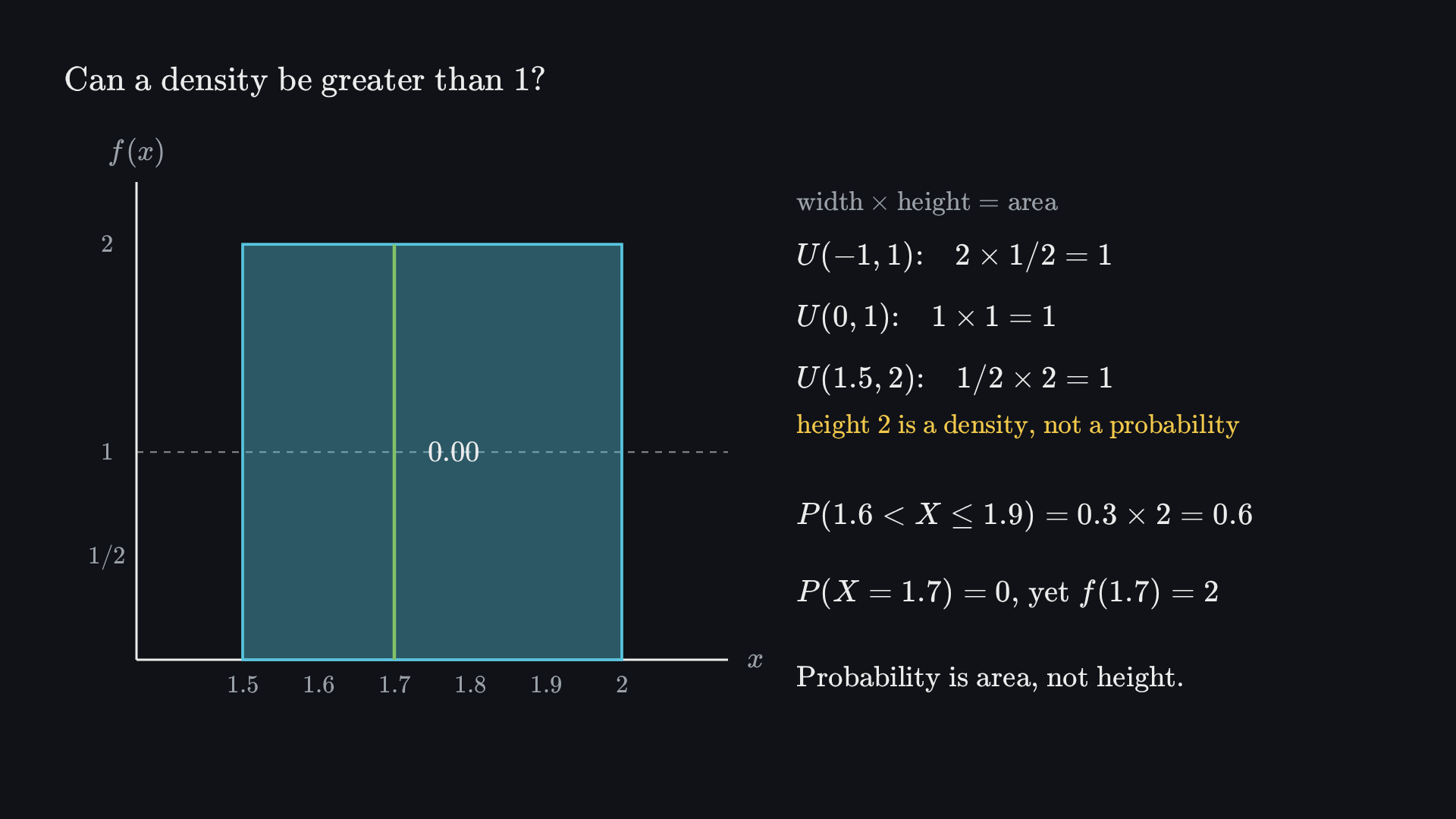
Shorter support requires a taller density
Every rectangle has area one. The density height changes inversely with support width, so the last height is two rather than a probability of two.
Distribution
Support width
Density height
Total area
U(0,1)
1
1
1
U(−1,1)
2
1/2
1
U(1.5,2)
1/2
2
1
For the last distribution, density 2 is compatible with probability one because its width is only 1/2. The interval from 1.5 to 1.75 has width 1/4, so its probability is 2(1/4)=1/2.
Before playing, predict: can a density be greater than 1? And what is the probability of one exact value?The animation’s final frame. Its numbered steps describe how the picture is built.
U(−1,1): a rectangle of width 2 and height 1/2 has area 1.
Squeeze the support to (0,1): the height doubles to 1 and the area stays 1.
Squeeze again to (1.5,2): height 2, area still 1. A height above 1 is allowed, because it is a density, not a probability.
Zoom in: the probability of (1.6,1.9] is its area, 0.3×2=0.6.
Shrink the interval to the point 1.7: its area, and so its probability, falls to 0 while the height stays 2.
For U(0,2), density is 1/2. The interval (0.8,1.5] has probability (1.5−0.8)/2=0.35. The cumulative probabilities at its endpoints are 0.4 and 0.75.
Interval area under a uniform density
The shaded width is 0.7 and the density height is one half, giving probability 0.35.
2.3.3A normal family has location and spread
The normal distribution, also called Gaussian, is a family of bell-shaped densities. Write X∼N(μ,σ2), where μ is its mean and σ>0 its standard deviation. The second parameter in this notation is the variance, σ2, not the standard deviation. Those measures are developed formally in the moments chapters.
One readable way to write the density introduces the standardized distance z=(x−μ)/σ:
zfX(x)=σx−μ,=σ2π1exp(−z2/2).
The exponential term decreases with squared distance from the centre. Dividing the distance by σ makes the same relative shape work at different scales; dividing the height by σ keeps the total area one when the horizontal scale expands.
Changing μ from −1 to 0 to 2, while keeping σ=1, shifts the curve without changing its spread. Keeping μ=0 and changing σ from 0.5 to 1 to 2 produces increasingly wide, lower curves. Their areas remain one; a lower peak does not mean that the total probability is smaller.
Shift location or change spread
Same spread
Same centre
Solid, dashed and dotted curves identify the listed parameter values in order. The vertical density scale is shared. Every curve integrates to one.
A normal distribution’s mathematical support is the entire real line. A bell shape alone does not establish that a measurement is normal, and the model can be inappropriate when hard boundaries or heavy tails matter. Normal probabilities describe areas, not curve heights. The next chapter supplies the cumulative function needed to calculate them.
2.3.4Density, height and probability
1. A height greater than one
Let X∼U(1.5,2). Find fX(1.7), P(1.6<X<1.9), and P(X=1.7).
Solution
Density height.fX(1.7)=1/(2−1.5)=2.
Interval area. Its width is 1.9−1.6=0.3, so the probability is 2(0.3)=0.6.
A point.P(X=1.7)=0, because the point has zero width. Density and probability answer different questions.
2. Clip to the support
For X∼U(−1,1), find P(−2<X≤0.5). Why is multiplying the full interval width by the density incorrect?
Solution
Retain supported values. Only [−1,0.5] contributes.
Area. Its width is 1.5 and density is 1/2, giving probability 0.75.
Check. The full width 2.5 would give 1.25, an impossible probability, because it includes values outside the support.
2.4 Cumulative distributions and quantiles
Thresholds, endpoints and reversing probability questions
2.4.1Accumulating probability up to a threshold
The cumulative distribution function, or CDF, answers one repeated question: what is the probability of a value no greater than a threshold? Define it for every real threshold x, including gaps in a discrete support:
FX(x)=P(X≤x).
For a discrete variable, add all masses at or below x. For a variable with a density, accumulate area from the far left up to x:
FX(x)FX(x)=u≤x∑pX(u),=∫−∞xfX(u)du.
These are alternative constructions for the discrete and density cases. The dummy variable u represents values being accumulated; x remains the chosen threshold.
For the ten-script pile, the cumulative masses at marks 30,60,80,90,100 are respectively 0.3,0.5,0.8,0.9,1. Between marks, nothing new is added. Thus FX(29.999)=0, FX(30)=0.3, FX(30.01)=0.3, and FX(70)=0.5. The function is a staircase, not a smooth curve.
A jump adds the probability at its mark
Filled points give the value at each threshold; open points show the excluded left limit. No new probability is added between supported marks.
At threshold 80, the retained marks have total mass 0.3+0.2+0.3=0.8. Immediately below 80, the cumulative mass is 0.5. The jump 0.3 is precisely the mass at 80.
Every CDF lies between zero and one, is nondecreasing, approaches zero far to the left, and approaches one far to the right. It is right-continuous: its value at a jump includes the mass at that threshold. A discrete CDF need not be continuous. For a distribution with a density, the CDF is continuous, but need not be differentiable at every point, as a uniform distribution’s endpoints illustrate.
2.4.2Interval probabilities and endpoint choices
An interval probability subtracts the mass already accumulated before the interval from the mass accumulated through its upper endpoint:
P(a<X≤b)P(X>x)=FX(b)−FX(a),=1−FX(x).
The first expression excludes a, because its mass is included in the subtracted FX(a). For discrete variables, changing an endpoint from strict to inclusive can change the answer. Write FX(a−) for the CDF limit just below a, read “F sub X at a from the left.” Then
P(a≤X≤b)=FX(b)−FX(a−),P(X=a)=FX(a)−FX(a−).
For the marks, P(30<X≤80)=0.8−0.3=0.5, whereas P(30≤X≤80)=0.8−0=0.8. The difference is the three scripts marked 30. For a variable with a density, endpoint masses are zero, so these strict and inclusive versions coincide.
For X∼U(a,b), accumulating the rectangle’s area gives
FX(x)=⎩⎨⎧0,b−ax−a,1,x<a,a≤x≤b,x>b.
For U(0,2), FX(0.8)=0.4 and FX(1.5)=0.75; their difference is 0.35. The same area can be found directly from width times height. Where the CDF is differentiable, its slope is the density: fX(x)=FX′(x). A steep CDF means probability accumulates quickly in that region, not that cumulative probability can exceed one.
2.4.3Reverse the question: quantiles
A probability calculation starts with a threshold and finds a probability. A quantile starts with a probability and finds a threshold. The p-quantile, for 0<p<1, can be defined by
QX(p)=inf{x:FX(x)≥p}.
Read inf as “infimum,” the lowest threshold satisfying the condition. For a continuous strictly increasing CDF this is the inverse function and solves FX(x)=p. The inequality definition also works at jumps, where no threshold may have exactly the requested cumulative probability.
The median corresponds to p=0.5; quartiles use 0.25,0.5,0.75; deciles use tenths; percentiles use hundredths. In a CDF plot, start at the requested probability on the vertical axis, move to the curve, then read the threshold on the horizontal axis. For a uniform distribution, solve the linear CDF:
pQX(p)=b−ax−a,=a+(b−a)p.
For the marks, the lower-quantile convention gives QX(0.25)=30, QX(0.5)=60, and QX(0.75)=80. A conventional sample median averages the fifth and sixth ordered records, giving (60+80)/2=70. These are different conventions for a distribution with a gap at its halfway point. Every value between 60 and 80 satisfies the usual median inequalities; specify the convention when a unique numerical answer is needed.
As a continuous example, a normal model N(5,4) has its 10th percentile near 2.44, first quartile near 3.65, median 5, third quartile near 6.35, and 90th percentile near 7.56. Standardisation will show how these numbers are obtained from one common reference distribution.
2.4.4Normal areas and table reading
For a standard normal variable Z∼N(0,1), write its CDF as Φ(z), pronounced “capital phi of z.” It is an S-shaped cumulative curve, while its density is bell-shaped. Normal areas have no elementary antiderivative; numerical routines or probability tables calculate them.
Selected standard normal cumulative probabilities
Threshold z
Φ(z)
−2.33
0.0099
−2
0.0228
−1.02
0.1539
−1
0.1587
−0.5
0.3085
0
0.5000
0.67
0.7486
0.68
0.7517
1
0.8413
1.96
0.9750
2
0.9772
In a two-dimensional table, a row such as 1.9 and a column such as 0.06 identify z=1.96. A negative-value table may use row −2.3 and column 0.03 to identify −2.33; inspect its sign convention. The entry is a left-tail probability, not a density height. At −2.33, that probability is about one percent, 0.0099, rather than 0.099.
Left tail.P(Z≤−1.02)=Φ(−1.02)=0.1539.
Right tail.P(Z≥1)=1−Φ(1)=0.1587. Normal symmetry also gives Φ(−1)=1−Φ(1).
Interval. For −0.5≤Z≤2, subtract the left tails:
P(−0.5≤Z≤2)=Φ(2)−Φ(−0.5)≈0.9772−0.3085=0.6687.
To find the third quartile from the table, 0.75 lies between 0.7486 at 0.67 and 0.7517 at 0.68. Linear interpolation uses the fraction of the probability gap traversed:
A more precise numerical inverse gives 0.674490. Interpolation is an approximation between rounded table entries, not a claim that the normal CDF is exactly linear there.
Quantiles and central intervals answer different questions
Question
Answer
7th percentile
−1.475791
87th percentile
1.126391
95th percentile; upper tail 0.05
1.644854
97.5th percentile
1.959964
Central 90%
Approximately ±1.645
Central 95%
Approximately ±1.96
Central 99%
Approximately ±2.5758
A central 95% interval leaves 2.5% in each tail. Its upper endpoint is therefore the 97.5th percentile, not the 95th. In particular P(∣Z∣≥1.645)≈0.10, while ±2.5758 describes a central 99% interval. These probabilities belong to the specified normal model.
2.4.5Work from the event to its cumulative probabilities
1. Endpoints in the mark distribution
Find P(60<X≤90), P(60≤X≤90), and P(X>80).
Solution
Exclude the lower endpoint.FX(90)−FX(60)=0.9−0.5=0.4.
Include it.FX(60−)=0.3, so 0.9−0.3=0.6.
Complement.P(X>80)=1−FX(80)=0.2.
2. A uniform quantile
Find the 75th percentile of U(−1,1), then check its CDF.
Solution
Inverse.x=−1+2(0.75)=0.5.
Check.FX(0.5)=(0.5+1)/2=0.75.
3. One tail or two?
Why does the normal 95th percentile not give an upper endpoint for a symmetric central 95% interval?
Solution
One-tail quantile. The 95th percentile leaves 5% above it.
Symmetry. Using its negative as the lower endpoint also leaves 5% below, so only 90% remains centrally.
Required tails. A central 95% interval needs 2.5% in each tail, giving endpoints about ±1.96.
2.5 Expected values
Probability-weighted averages and transformations
2.5.1The mean is a probability-weighted balance
A distribution records the full allocation of probability. An expected value summarizes its location by weighting each value according to how much probability it receives. “Expectation,” “mean” and “expected value” refer to the same mathematical object. Expectation does not mean the outcome that will occur, or necessarily the outcome that occurs most often.
Definition. For a finite expected value, assume E[∣X∣]<∞. Then
For a discrete distribution,
E[X]=x∑xpX(x).
For a distribution with a density,
E[X]=∫−∞∞xfX(x)dx.
Values with more probability exert more influence; impossible values exert none. The integrability condition prevents infinite positive and negative contributions from being treated as if they cancelled. All finite-support examples here satisfy it.
For the ten-script pile, averaging individual marks and averaging distinct marks with their probabilities give the same result:
The individual records sum to 640, so their ordinary mean is also 640/10=64. Grouping repeated marks changes the calculation’s organization, not its result. The mean is the balance point of the probability weights: E[X−μ]=0.
The mean need not be a supported value
The dashed line locates the probability-weighted mean; the stems remain at the five possible marks. Values on both sides balance in their weighted deviations.
No script has mark 64, yet it is the expected mark of a uniform selection. A fair die likewise has mean (1+2+3+4+5+6)/6=3.5, which is not a possible face. The modes of the mark distribution are 30 and 80, each with probability 0.3; neither equals the mean. These examples separate an average from a prediction of one exact outcome.
2.5.2Indicators and continuous averages
For a Bernoulli indicator with P(X=1)=p,
E[X]=0(1−p)+1p=p.
Its expectation is the probability of the event coded one. For the blue-eye indicator record 1,0,0,1,1,0,1,0,0,0, four of ten entries are one. Its mean is 0.4, the proportion coded blue-eyed. This is an average of indicators, not an average eye colour.
For a uniform variable, the mean is its midpoint. Derive it by weighting each value with the constant density:
E[X]=b−a1∫abxdx=2(b−a)b2−a2=2a+b.
Thus U(10,20) has mean 15. For N(μ,σ2), the mean is μ. Its density is symmetric about μ, so equal probability weights at opposite distances cancel in the expectation of X−μ. This argument relies on the mean existing; symmetry alone is not sufficient.
2.5.3Transform values first, then average
For a function g, the expectation of the transformed measurement is found using the original probability weights:
E[g(X)]E[g(X)]=x∑g(x)pX(x),=∫g(x)fX(x)dx.
The first expression is for discrete values and the second for a density. This method avoids constructing the transformed distribution when only its average is required. It also makes clear that averaging and transforming are two separate operations.
Squaring the mean instead gives 642=4096. The difference comes from variation around the mean. It will become the variance in the next chapter.
Linearity. For constants a,b and integrable variables,
E[a+bX]E[X+Y]=a+bE[X],=E[X]+E[Y].
Expand the weighted sum. Each term of E[a+bX] is (a+bx)pX(x).
Separate terms. Sum the constant part and the variable part separately.
Normalize. The constant part is a∑xpX(x)=a; the remaining part is bE[X].
The same separation works for integrals and for sums of variables. Addition does not require independence. Multiplication is different: independence gives E[XY]=E[X]E[Y], when the required expectations exist. Without that condition, the joint distribution determines the average product. More generally, independent variables also allow E[g(X)h(Y)]=E[g(X)]E[h(Y)] under integrability.
For N binary trials with common success probability p, linearity gives E[∑iXi]=Np and E[Xˉ]=p. Independence is unnecessary for these two mean identities; it is needed for the binomial distribution of the count.
2.5.4Nonlinearity and the existence of moments
A convex function bends upward: a straight segment joining two points on its graph lies on or above the graph. A concave function reverses that geometry. Jensen’s inequality, pronounced “YEN-sen’s inequality,” extends that comparison to probability-weighted averages, assuming the relevant expectations exist:
For convex g,
E[g(X)]≥g(E[X]).
For concave g,
E[g(X)]≤g(E[X]).
Squaring and exponentiation are convex; logarithms on positive values and square roots on nonnegative values are concave. Consequently E[X2]≥(E[X])2, E[eX]≥eE[X], E[logX]≤logE[X] for positive X, and E[X]≤E[X] for nonnegative X. Equality can occur, for example when there is no variation; “nonlinear” does not automatically mean every instance is strictly unequal.
Ratios also need care. Suppose two paired outcomes (X,Y)=(1,1) and (1,2) are equally likely. Then E[X/Y]=(1+1/2)/2=3/4, while E[X]/E[Y]=1/(3/2)=2/3. Averaging ratios is not generally the same as taking the ratio of averages.
Why a symmetric density can have no mean
The standard Cauchy density is f(x)=1/[π(1+x2)]. Its tails decrease much more slowly than normal tails. Its positive first-moment integral contains
∫0∞1+x2xdx,
which diverges, since an antiderivative is 21log(1+x2). The negative side also has infinite magnitude. Symmetric cancellation in a principal-value calculation is not a finite expectation; the Cauchy mean and variance do not exist. A distribution’s plausible-looking central shape does not establish the existence of its moments or the rarity of its extreme observations.
2.5.5Choose the correct order of operations
1. An affine change of marks
The marks are transformed by Y=5+0.8X. Find E[Y]. Is independence relevant?
Solution
Linearity.E[Y]=5+0.8E[X].
Use the existing mean.5+0.8(64)=56.2.
Assumptions. This is a function of one variable; linearity, not independence, justifies the calculation.
2. Square before averaging
For a fair die, find E[X2] and compare it with (E[X])2.
Solution
Average transformed values.E[X2]=(1+4+9+16+25+36)/6=91/6.
Transform the average.(E[X])2=(7/2)2=49/4.
Compare. Their difference is 91/6−49/4=35/12>0, consistent with convexity of squaring.
3. Does an expected value have to be possible?
A payoff is 0 with probability 0.9 and 100 with probability 0.1. Find its mean and mode.
Solution
Weighted mean.0(0.9)+100(0.1)=10.
Most likely value. The mode is 0.
Interpretation. The mean 10 is a probability-weighted summary, despite not being a possible payoff.
2.6 Variance and standard deviation
Squared deviations, units and spread
2.6.1Why square deviations?
Two distributions can have the same mean and very different spread. Ordinary deviations cannot summarize spread by their average, because positive and negative deviations from the mean cancel: E[X−μ]=0. Squaring prevents that cancellation, weights larger deviations more strongly, and produces a nonnegative summary.
Definition. With finite second moment and μ=E[X],
Var(X)=E[(X−μ)2].
Read “variance of X.” This is the second central moment. The raw second moment is E[X2]; it is related to variance but is not the same object.
Expand the square.(X−μ)2=X2−2μX+μ2.
Apply linearity. The fixed μ can be taken outside the expectation.
Substitute the mean. Since E[X]=μ,
Var(X)=E[X2]−2μE[X]+μ2=E[X2]−μ2.
For a PMF, variance is ∑x(x−μ)2pX(x); for a density, it is ∫(x−μ)2fX(x)dx. Its nonnegativity follows directly from averaging squared deviations. A finite-variance variable has variance zero exactly when it equals a constant with probability one.
The standard deviation is the square root:
σ=SD(X)=Var(X).
The mean is in the variable’s original units; variance is in squared units; standard deviation returns to the original units. For income measured in pounds, variance is in pounds squared and standard deviation is in pounds.
2.6.2The same marks, now measuring spread
For the mark distribution, μ=64, E[X2]=4720, and μ2=4096. Therefore
Var(X)SD(X)=4720−4096=624,=624≈24.98.
Direct weighted-deviation check
Mark x
Deviation x−64
Weighted square
30
−34
0.3(342)=346.8
60
−4
0.2(42)=3.2
80
16
0.3(162)=76.8
90
26
0.1(262)=67.6
100
36
0.1(362)=129.6
Total
624
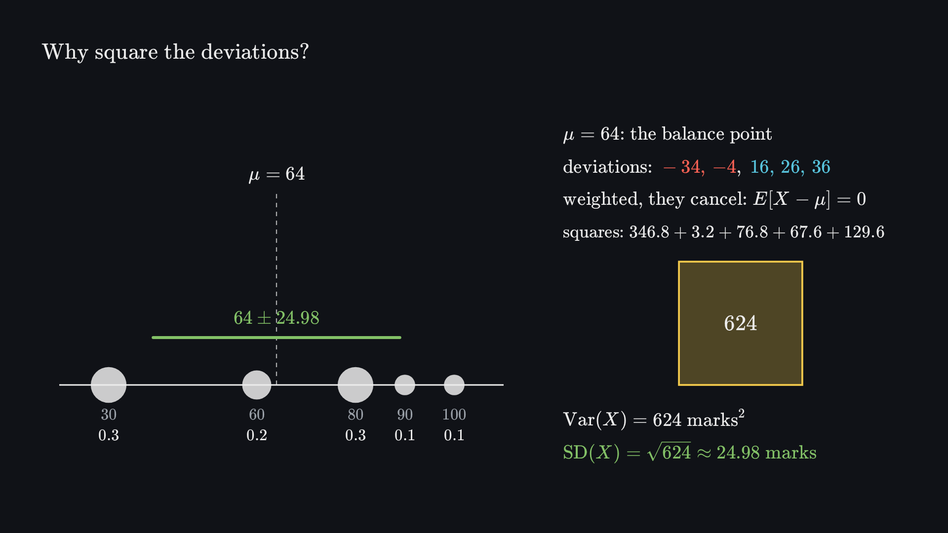
Before playing, predict: what is the probability-weighted average of the deviations from the mean, 64? Why can it not measure spread?The animation’s final frame. Its numbered steps describe how the picture is built.
Five marks with probabilities 0.3,0.2,0.3,0.1 and 0.1 balance at their mean, 64.
Their deviations, −34,−4,16,26 and 36, cancel once weighted by probability: E[X−μ]=0.
Squaring stops the cancelling: each deviation becomes a square, which then shrinks to its probability share.
The weighted squares, 346.8+3.2+76.8+67.6+129.6, pool into one square of area 624 marks²: the variance.
Its side, 624≈24.98 marks, is the standard deviation, back in the original units: 64±24.98.
This variance describes a uniform draw from the known pile of ten scripts, so the record-based calculation divides by ten. An estimator of an unknown population variance from a random sample may use a different denominator. That later estimation problem should not be confused with the variance of this fully specified distribution.
For a change of units Y=a+bX, the mean becomes a+bμ. Its deviation is Y−E[Y]=b(X−μ), so
Var(a+bX)SD(a+bX)=b2Var(X),=∣b∣SD(X).
A shift changes location without changing spread. Multiplication changes spread by the magnitude of the multiplier; a negative multiplier also reverses order. If marks were expressed as proportions rather than percentages, the standard deviation would be 24.98/100, while variance would be 624/1002.
2.6.3Variances of useful distributions
For a Bernoulli variable with success probability p, the identity X2=X holds because its only values are zero and one. Hence
Var(X)=E[X2]−(E[X])2=p−p2=p(1−p)=41−(p−21)2.
The variance is zero when all probability is on one outcome and largest at p=1/2. Knowing a binary variable’s mean determines its variance, and indeed its whole Bernoulli distribution. For general numerical variables, knowing the mean alone does not determine spread.
For U(a,b), write L=b−a and centre the variable at (a+b)/2. Its deviations are uniform from −L/2 to L/2, so
Var(X)=L1∫−L/2L/2u2du=12L2=12(b−a)2.
Thus U(10,20) has variance 100/12 and standard deviation 10/12≈2.887. For N(μ,σ2), the parameters are directly its mean and variance. The notation is consistent across normal probability calculations: use σ=σ2 when dividing a distance by standard deviation.
For independent Bernoulli trials, the variance of their sum is Np(1−p). Independence makes the cross-covariance terms vanish; the association chapter will derive the general sum-variance rule. The variance of their average is p(1−p)/N, explaining why a proportion can concentrate even while the success count’s numerical spread grows with N.
2.6.4Standard deviation as a common distance unit
When σ>0, the standardized measurement is Z=(X−μ)/σ. Its mean is zero and variance one. A value of 1 is one standard deviation above the mean; a value of −2 is two below. This change of units works for any finite positive variance, but it does not turn every distribution into a normal distribution.
For a normal model, central probabilities are approximately 68.27% within one standard deviation, 95.45% within two, and 99.73% within three. This is often called the empirical rule. A central 95% normal interval uses about 1.96 standard deviations, rather than exactly two. A six-standard-deviation event is exceptionally rare under a normal model, but its rarity cannot be inferred from the number of standard deviations alone if the distribution has heavy tails.
The next chapter combines this common unit with the standard normal CDF to calculate probabilities and quantiles. Keep two questions separate: how far a value lies from the mean in standard deviations, and how much probability the assumed distribution puts beyond that distance.
2.6.5Spread and transformations
1. Shift and scale
For the mark distribution, define Y=10−2X. Find its mean, variance and standard deviation.
Solution
Mean.E[Y]=10−2(64)=−118.
Variance.Var(Y)=(−2)2(624)=2496.
Standard deviation.SD(Y)=2624≈49.96. A negative scale cannot create a negative spread.
2. A binary distribution
A Bernoulli variable has mean 0.9. Find its variance. Compare it with a Bernoulli variable of mean 0.5.
Solution
Identify the success probability.p=E[X]=0.9.
Variance.0.9(0.1)=0.09.
Comparison. At p=0.5, variance is 0.25. The distribution near all successes is less variable than the half-and-half distribution.
2.7 Normal standardisation
Translate probabilities and quantiles between scales
2.7.1Translate a normal model without changing the event
Standard normal probabilities can serve every normal distribution because shifting and scaling a normal variable preserves its normal shape. If X∼N(μ,σ2) and Y=a+bX, with b=0, then
Y∼N(a+bμ,b2σ2).
The new mean follows linearity of expectation; the new variance follows the squared-deviation rule. The standard deviation is ∣b∣σ. With b=0, the result is a constant rather than a variable with a nondegenerate normal density.
Track the two normal parameters separately
Starting model
Transformation
Result
N(5,4)
X+10
N(15,4)
N(5,4)
X−5
N(0,4)
N(1,2)
2X
N(2,8)
N(1,2)
−3X
N(−3,18)
Subtracting the mean centres a normal variable without altering variance. Dividing by standard deviation then sets the variance to one:
X−μZ=σX−μ∼N(0,σ2),∼N(0,1).
Read Z as a new random variable; read z=(x−μ)/σ as the transformed numerical threshold. The distinction matters: standardising the distribution and standardising the event’s endpoints are two parts of the same operation.
2.7.2Probabilities: preserve the inequality and choose its area
Because σ>0, subtracting μ and dividing by σ preserves an inequality’s direction. Therefore
P(X≤x)P(X≥x)=Φ(σx−μ),=1−Φ(σx−μ).
For an interval, transform both endpoints and subtract their left-tail probabilities. Dividing by a negative multiplier in some other transformation would reverse inequalities; standardisation itself uses a positive standard deviation.
Example 1: a left tail
Let X∼N(−1,9). The standard deviation is 3, not 9. For P(X≤2),
zP(X≤2)=32−(−1)=1,=Φ(1)≈0.8413.
The threshold is one standard deviation above the mean. A probability above one half is consistent with its location.
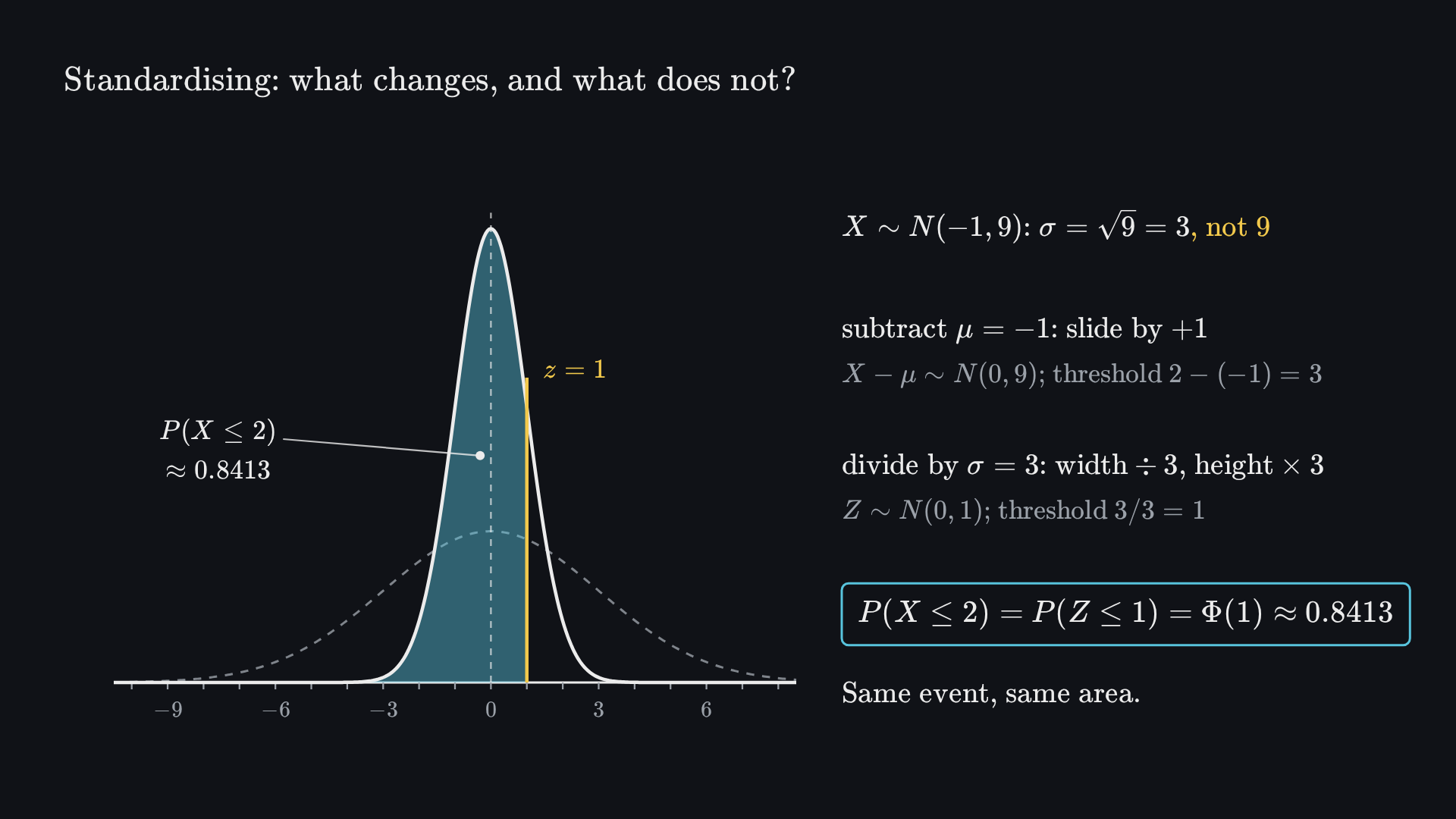
Before playing, predict: to standardise X∼N(−1,9), do we divide by 9 or by 3? And does the shaded area change?The animation’s final frame. Its numbered steps describe how the picture is built.
X∼N(−1,9) has σ=9=3, not 9. The probability P(X≤2) is the shaded area.
Subtract the mean μ=−1: the curve and the threshold slide together by +1. Now X−μ∼N(0,9) and the threshold is 2−(−1)=3.
Divide by σ=3: the curve becomes three times narrower and three times taller, and the threshold becomes 3/3=1. The shaded area does not change.
So P(X≤2)=P(Z≤1)=Φ(1)≈0.8413: the threshold is one standard deviation above the mean.
Example 2: keep track of table rounding
For X∼N(4,1/2), find P(X≤3.5):
σzP(X≤3.5)=1/2,=1/23.5−4≈−0.707107,≈0.23975.
Rounding the standardized threshold first to −0.71 and using a two-decimal table gives 0.2389. The difference is rounding, not a different model. Keep unrounded values for numerical calculations and state the approximation when using a table.
The two bounds surround the mean. Draw or identify that central segment before subtracting; the interval is zlower≤Z≤zupper, with both inequalities pointing consistently.
For N(0,1), the interval from −0.5 to 2 has probability Φ(2)−Φ(−0.5)≈0.6687. Altering mean or variance requires transforming both original endpoints before using those cumulative probabilities.
The interval is a difference of left-tail areas
The shaded interval has probability about 0.6687. Its endpoints must be translated to standardized distances before this curve can represent an interval from a different normal model.
2.7.3Quantiles: transform back into original units
Given a probability p, first find its standard normal quantile zp=Φ−1(p), read “phi inverse of p.” Then undo the standardisation:
zpxp=σxp−μ,=μ+σzp.
A normal distribution’s median is its mean, because z0.5=0. Thus the median of N(−1,9) is −1. For the third decile of N(4,1/2), use p=0.3:
A quantile below the median should be below the mean, a useful direction check. For N(5,4), standard deviation is 2; transforming the standard quantiles gives the earlier values 2.44,3.65,5,6.35,7.56 at probabilities 0.1,0.25,0.5,0.75,0.9.
A reliable calculation follows four steps: write the event or requested probability; distinguish variance from standard deviation; translate the threshold or probability to the standard normal; translate the final answer back if the question asks for a value. A probability has no measurement units; a quantile has the variable’s units.
2.7.4Calculate and check the direction
1. An upper tail
Let X∼N(5,4). Find P(X>7).
Solution
Scale.σ=4=2.
Threshold.z=(7−5)/2=1.
Upper tail.P(X>7)=1−Φ(1)≈0.1587.
Check. A threshold above the mean has an upper-tail probability below one half.
2. A central interval in original units
Find an approximately central 95% interval for N(−1,9).
Solution
Standard endpoints. Central 95% uses approximately −1.96 and 1.96.
Transform back. Multiply by 3, then add −1.
Result. The interval is [−6.88,4.88]. Using the 95th percentile 1.645 instead would leave only 90% centrally.
3. Standardized does not mean normal
Does (X−E[X])/SD(X) have a standard normal distribution whenever the standard deviation is positive?
Solution
No. It has mean zero and variance one, but retains the original distribution’s shape under the affine change. Standardising a uniform variable gives another uniform variable, not a bell curve. Normality of X is the assumption that permits standard normal probability calculations.
2.8 Joint, marginal and conditional distributions
Pair measurements, integrate margins and normalize slices
2.8.1Keep paired measurements together
A joint distribution describes measurements made together. For two dice, X might be the first die and Y the second. An outcome is a pair, not two unrelated lists. In a class record, a mark and a group indicator must refer to the same student if their relationship is to be studied.
Joint cumulative distribution.
FX,Y(x,y)=P(X≤x,Y≤y).
The comma means both inequalities hold. It accumulates probability in the region below both thresholds. For discrete variables, the joint PMF is pX,Y(x,y)=P(X=x,Y=y). It is nonnegative and its sum over all pairs is one:
x∑y∑pX,Y(x,y)=1.
For a joint density fX,Y, interval rectangles receive probabilities by integration:
P(a<X≤b,c<Y≤d)=∫ab∫cdfX,Y(x,y)dydx.
A joint density’s total volume is one, and a single pair has zero probability. When the cumulative function is sufficiently differentiable, fX,Y(x,y)=∂2FX,Y(x,y)/(∂x∂y).
For two independent fair dice, all 36 pairs have mass 1/36. The joint probability P(X≤2,Y≤3) contains six pairs, so it is 6/36=1/6. Different joint distributions can have the same individual distributions: knowing each die’s separate probabilities does not determine how their values are paired.
Joint cells, marginal totals
Columns identify the first die and rows the second. Each cell is one paired outcome. Adding a row or a column gives a marginal probability of one sixth; selecting a row and normalizing gives a conditional distribution.
2.8.2Marginalise by adding over the other measurement
A marginal distribution describes one variable without conditioning on the other. To obtain it, retain every possible value of the other coordinate and add their joint probabilities. The name is reflected in a table: its row and column totals sit in the margins.
pX(x)pY(y)=y∑pX,Y(x,y),=x∑pX,Y(x,y).
For a continuous joint density, sums become integrals:
Marginalising is not the same as slicing. A slice fixes a coordinate; a marginal combines its whole range. For the independent fair dice, a row has six cells of mass 1/36, giving a marginal mass 1/6. A column gives the same result for the other die.
Variables are independent when their joint probabilities factor into marginal probabilities for all relevant events. For discrete values this is pX,Y(x,y)=pX(x)pY(y). For densities the analogous factorisation holds almost everywhere, and for cumulative functions it is FX,Y(x,y)=FX(x)FY(y). Checking one cell is insufficient to establish independence; the relationship must describe the whole distribution.
2.8.3A conditional distribution is a normalized slice
In a discrete model, conditioning on a value with positive marginal probability uses the familiar event ratio:
pY∣X(y∣x)=pX(x)pX,Y(x,y).
The numerator keeps the slice at the selected X value; division by its X-marginal probability makes the conditional masses sum to one. In the dice grid, that slice is a column because X labels the horizontal axis. For independent dice, the numerator is 1/36 and the denominator 1/6, so the conditional mass remains 1/6: learning one die’s value does not change the other die’s distribution.
For variables with a joint density, the corresponding conditional-density construction is, where fX(x)>0,
fY∣X(y∣x)=fX(x)fX,Y(x,y).
This is a density construction, not division by the point probability P(X=x), which is zero. The raw slice has area fX(x); dividing by that area normalizes it. Conditional densities can be specified at suitable conditioning values, or almost everywhere, without applying the elementary event ratio to a zero-probability event.
A geometric model where the slice changes
As an explicit hypothetical model, take constant joint density 2 on the triangle 0<x<y<1, and zero elsewhere. Its triangular area is 1/2, so total probability is 2(1/2)=1.
Integrate a slice, then normalize it
The triangle carries constant density two, so its total volume is one. The horizontal segment at Y equal to three quarters has width three quarters: its raw slice integrates to three halves and its conditional density is four thirds.
Marginal of Y. At a fixed y, the horizontal slice runs from x=0 to x=y, giving fY(y)=∫0y2dx=2y, for 0<y<1.
Conditional density of X. Divide that slice by its total: fX∣Y(x∣y)=2/(2y)=1/y, for 0<x<y.
Interpretation.X∣Y=y is uniform from zero to y. Increasing the known y permits a wider range of X, rather than leaving its distribution unchanged.
Other marginal. Fixing x and integrating from y=x to one gives fX(x)=2(1−x), for 0<x<1.
At y=1/2, the conditional density is 2 over width 1/2; at y=3/4, it is 4/3 over width 3/4. Both areas are one. The joint density is not the product of these marginals, so the variables are dependent. Two-dimensional geometry helps distinguish a volume, an integrated marginal, and a renormalized slice without requiring a three-dimensional perspective drawing.
2.8.4A joint table for the original class
To connect distributions with group averages, now let Y denote a student’s mark and X the class record’s group indicator: 1 for women and 0 for men. The earlier mark variable has been renamed Y; the values have not changed. Pair the ten marks with the recorded indicator sequence 0,0,0,1,1,0,1,0,1,0. Uniformly selecting a student gives:
Joint probabilities from paired class records
Mark y
X=0
X=1
Mark marginal
30
0.3
0
0.3
60
0
0.2
0.2
80
0.2
0.1
0.3
90
0
0.1
0.1
100
0.1
0
0.1
Group marginal
0.6
0.4
1
For example, P(Y=80∣X=1)=0.1/0.4=1/4, while P(Y=80∣X=0)=0.2/0.6=1/3. The numerator represents a joint group–mark event, not the whole mark marginal 0.3. Marginalizing across groups recovers the original mark distribution; conditioning on a group creates a different normalized mark distribution. The conditional-expectation chapter will average these distributions.
2.8.5Marginal, conditional or joint?
1. One cell and one margin
Using the class table, find P(Y=60), P(X=1,Y=60), and P(X=1∣Y=60).
Solution
Mark marginal. Add across groups: 0+0.2=0.2.
Joint cell. The group-one, mark-sixty cell is 0.2.
Conditional. Divide by the mark-sixty marginal: 0.2/0.2=1. In this pile, every mark-sixty script belongs to group one.
2. A normalized slice
In the triangular density model, find P(X<1/4∣Y=1/2).
Solution
Conditional model.X∣Y=1/2 is uniform on (0,1/2), with density 2.
Interval area.2(1/4)=1/2.
Distinction. This conditional-density calculation does not use P(Y=1/2) as a denominator.
2.9 Conditional expectations
Group averages, weights and iterated expectation
2.9.1Average a distribution after conditioning
A conditional expectation is the mean of a conditional distribution. It answers a question such as: among members of this group, what is the average outcome? Keep the class notation Y for mark and X for its group indicator.
For a fixed value x, assuming the relevant conditional mean exists,
The second line is the discrete case and the third the density case. First restrict and normalize the distribution, then average it. The weights must sum to one within the chosen group.
The distinction between m(x) and m(X) is useful. At a particular known group, its mean is a number. Before we know which group a selected student belongs to, the conditional mean is itself a variable: it takes the appropriate group mean when X is realized. It predicts a group average, not every individual’s exact mark.
Conditional means are central to regression and comparisons between groups. For an income variable Y, a difference between means conditional on a recorded gender indicator describes an average earnings gap. It does not by itself measure what changing gender would cause, because the groups can differ in other relevant features. Causal interpretation requires the assumptions developed in the causal topic.
2.9.2Group means retain the original students
The four group-one marks are 60,60,80,90. The six group-zero marks are 30,30,30,80,80,100. Their conditional means are
The group totals are 290 and 350, respectively. Dividing each by its own number of students gives
Equivalently, the conditional probabilities within group one are 1/2 at 60, 1/4 at 80, and 1/4 at 90. Their weighted average is again 72.5. The between-group mean difference is 72.5−175/3=85/6≈14.1667, an association in these records.
The unweighted mean of the two group means is approximately 65.4167, not the overall mean 64. Giving each group equal weight would describe a population split equally between the groups, whereas the actual class shares are 0.4 and 0.6. Each student should have equal weight in a uniform draw from the class, not each group.
At the original share P(X=1)=0.4, the two group contributions are 0.4(72.5)=29 and 0.6(175/3)=35. Their sum is 64. A hypothetical half-and-half mixture would instead have mean 65.4167, holding the two group distributions fixed.
An overall mean lies between group means
The point is four tenths of the distance from group-zero mean to group-one mean. Equal group weighting would place it halfway, describing a different mixture.
2.9.3The law of iterated expectation
Law of iterated expectation. For an integrable Y,
E[Y]=E[E[Y∣X]].
Average within each group, then average the group means using their probabilities. The outer expectation averages over X; the inner expectation averages over Y conditional on that X.
Conditional mean. Define m(x)=∑yypY∣X(y∣x).
Weight by group probability. Average m(x) over the distribution of X.
Restore joint weights. Multiplication by pX(x) turns each conditional mass into pX,Y(x,y).
Marginalize. Sum those joint masses over x to recover the marginal distribution of Y.
For the class this gives, without rounding the group mean prematurely,
E[Y]=0.4(72.5)+0.6(175/3)=29+35=64.Before playing, predict: the two group means are 72.5 and 58.33. Is the class mean their simple average, 65.42?The animation’s final frame. Its numbered steps describe how the picture is built.
Ten students, one dot each. The class mean is E[Y]=640/10=64.
Split the class by X and average within each group: E[Y∣X=1]=290/4=72.5 and E[Y∣X=0]=350/6≈58.33.
Replace each mark by its group mean. This is E[Y∣X]:72.5 for 4 of the 10 students and 58.33 for the other 6, so the weights are 0.4 and 0.6.
Average with those weights: 0.4(72.5)+0.6(175/3)=29+35=64=E[Y]. The simple average 65.42 would weight the groups equally, as if the class were split half and half.
The same logic works with densities and integrals. Zero-probability groups contribute no joint mass; elementary conditional ratios need only be formed for positive-probability groups.
2.9.4What can be treated as known?
When conditioning on X, any function of X is known within that condition. For suitable integrable quantities,
E[h(X)Y∣X]=h(X)E[Y∣X].
At X=x, the multiplier h(x) is fixed, so it comes outside the conditional average just as a constant comes outside an ordinary expectation. This does not permit pulling an unknown function of Y outside an expectation conditioned only on X.
If X and Y are independent, the conditional distribution of Y does not change with X, so E[Y∣X]=E[Y]. The reverse implication is weaker: an unchanged conditional mean does not establish an unchanged whole distribution. Conditional variance or other features might still vary. The next chapter distinguishes full independence, mean-independence and zero covariance.
In the triangular density model, X∣Y=y was uniform from zero to y. Its conditional mean is therefore y/2. This is a continuous conditional-mean function: a larger value of the conditioning variable changes the expected value of the other measurement. The function can be meaningful even though each exact conditioning point has zero probability in an unconditional continuous model.
2.9.5Restore the population weights
1. A hypothetical mixture
Hold the two class group distributions fixed but give group one population share 0.7. What is the mixture mean?
Interpretation. The mixture changes because group proportions change. The original class remains a different distribution with mean 64.
2. Pull out what is known
In the original class, find E[XY∣X=0], E[XY∣X=1], and E[XY].
Solution
Condition zero.X is zero, so the product and its conditional mean are zero.
Condition one.X is one, so E[XY∣X=1]=E[Y∣X=1]=72.5.
Average across groups.E[XY]=0.6(0)+0.4(72.5)=29.
2.10 Covariance, correlation and independence
Separate linear association from probabilistic dependence
2.10.1Measure whether deviations move together
Variance squares one variable’s deviation. Covariance multiplies deviations of two variables measured together. Assume finite second moments, and write their means as μX=E[X] and μY=E[Y].
Definition.
Cov(X,Y)=E[(X−μX)(Y−μY)].
If both deviations have the same sign, their product is positive. If one is above its mean while the other is below, their product is negative. Covariance averages these signed products using the joint distribution. A positive result indicates a tendency for above-average values to occur together; a negative result indicates an opposite tendency. It does not assert that every pair follows that pattern.
Products of deviations determine the sign
Pairs in the upper-right and lower-left contribute positively; pairs in the other two quadrants contribute negatively. Covariance is the weighted average of these products, including their magnitudes.
Expand. The product is XY−μXY−μYX+μXμY.
Average. Apply linearity and substitute both means.
Cancel constants. This gives
Cov(X,Y)=E[XY]−E[X]E[Y].
Covariance is often denoted σXY, read “sigma sub X Y.” Its units are the product of the two measurement units, so changing units changes its numerical magnitude. Setting X=Y recovers Var(X).
For the class, retain X as the binary group indicator and Y as mark. We found E[X]=0.4, E[Y]=64, and E[XY]=29. Thus Cov(X,Y)=29−0.4(64)=3.4. The positive covariance reflects the higher mean mark in group one; it is descriptive rather than a causal effect.
2.10.2Covariance rules and the spread of sums
Covariance is symmetric, unchanged by adding constants to either variable, and linear in each argument separately. For constants a,b,c,d,
It also distributes across addition: Cov(X,Y+Z)=Cov(X,Y)+Cov(X,Z). These properties are called bilinearity. They follow by centring the variables, pulling constants outside expectations, and separating sums.
To calculate the variance of a sum, square its combined deviation:
The formula with subtraction follows by replacing b with −b. Positive covariance increases the spread of a sum but reduces the spread of a difference. Dropping the covariance terms requires a justification. Independence is sufficient; zero covariance is sufficient for this variance calculation even when the variables are dependent.
2.10.3Correlation removes the units
When both standard deviations are positive, define correlation by
ρXY=Corr(X,Y)=σXσYCov(X,Y).
It is the covariance of the standardized variables. Removing their units lets the same measure compare relationships expressed on different positive scales. In the class, Var(X)=0.4(0.6)=0.24 and Var(Y)=624, so
ρXY=0.246243.4≈0.27783.
Correlation lies between −1 and 1. To see why, let ZX,ZY be the standardized variables. Their variances are one, so nonnegativity of Var(ZX−ZY)=2−2ρ gives ρ≤1, and nonnegativity of Var(ZX+ZY)=2+2ρ gives ρ≥−1. Equality describes an exact linear relationship with probability one. Positive changes of units preserve correlation; reversing one variable’s sign reverses its sign.
If either variable has zero variance, covariance is zero but correlation is undefined because its denominator is zero. It should not be reported as zero correlation. Correlation summarizes linear association; zero correlation does not establish the absence of every relationship.
2.10.4Independence, mean-independence and zero covariance
Full independence means learning one variable does not change the other’s whole distribution. With the required finite moments, independence implies E[XY]=E[X]E[Y], hence zero covariance and, when both variances are positive, zero correlation. The reverse implications need not hold.
A concrete hypothetical model exposes the distinction. Let X take −1,0,1 with equal probabilities and define Y=X2. Then
E[X]=0,E[Y]=2/3,E[XY]=(−1+0+1)/3=0,Cov(X,Y)=0.
The correlation is also zero because both variances are positive. Nevertheless, Y is completely determined by X. For example P(Y=0∣X=0)=1, whereas P(Y=0)=1/3. The positive and negative contributions to covariance cancel; the relationship has not disappeared.
Zero correlation can arise from different joint models
Deterministic quadratic
Independent values
Both models have zero correlation. In the first, knowing X completely determines Y; in the second, learning X leaves every Y probability unchanged. Each point has equal probability within its panel.
For the three equally likely pairs (−1,1),(0,0),(1,1), covariance and correlation are zero, but Y=X2 is deterministic. An independent model with all nine pairs from {−1,0,1}2 equally likely also has zero correlation, for a different reason.
Mean-independence asks only whether a conditional mean changes. Y is mean-independent of X when E[Y∣X]=E[Y]. X is mean-independent of Y when E[X∣Y]=E[X]. These are different directional conditions; one need not imply the other.
In the quadratic example, E[X∣Y=0]=0, and at Y=1 the values −1 and 1 are equally likely, giving E[X∣Y=1]=0. Thus X is mean-independent of Y. But E[Y∣X]=X2 varies, so Y is not mean-independent of X. Full independence would imply both directions.
Mean-independence implies zero covariance under the relevant moment conditions: if E[Y∣X]=E[Y], then iteration and pulling out the known X give E[XY]=E[XE[Y∣X]]=E[X]E[Y]. Zero covariance alone does not imply this conditional-mean equality. For example, take equal probabilities on X=−2,−1,1,2 and set Y=X4. Symmetry gives E[X]=0 and E[XY]=E[X5]=0, so covariance is zero. Yet E[Y∣X]=X4 changes with X. For either Y=1 or Y=16, X has equally likely opposite signs, so E[X∣Y]=0=E[X]. Only the reverse directional mean-independence holds.
These distinctions describe progressively weaker aspects of a joint distribution. None supplies a causal interpretation by itself. The appropriate notion depends on the question: calculating a sum’s variance, predicting a conditional mean, and asserting full probabilistic independence require different evidence.
2.10.5State the needed condition
1. Covariance changes a sum
Suppose Var(X)=4, Var(Y)=9, and Cov(X,Y)=3. Find Var(X+Y), Var(X−Y), and correlation.
Solution
Sum.4+9+2(3)=19.
Difference.4+9−2(3)=7.
Standardize covariance.ρ=3/(49)=1/2. Both standard deviations are positive, so the ratio is defined.
2. A constant variable
If X=5 with probability one and Y has finite positive variance, what are covariance and correlation? Is X independent of Y?
Solution
Centre the constant.X−E[X]=0, giving covariance zero.
Correlation. It is undefined because σX=0.
Independence. A constant variable is independent of every other variable: knowing it supplies no uncertain measurement information. This does not repair the zero denominator in correlation.
3. Uncorrelated does not mean unrelated
For the equal-probability quadratic model X∈{−1,0,1}, Y=X2, find both variances and explain why zero covariance does not prove independence.
Solution
Variance of X.E[X2]=2/3 and its mean is zero, so variance is 2/3.
Variance of Y.Y2=Y, giving 2/3−(2/3)2=2/9.
Conditional distribution.X=0 forces Y=0, while its marginal probability is only 1/3. Independence fails despite zero covariance and correlation.
![Final frame: three number lines. On the rows X = 1 and X = 0, balance points mark the group means 72.5 (marks 60, 60, 80, 90) and 58.33 (marks 30, 30, 30, 80, 80, 100). On the bottom line, a stack of 6 dots at 58.33 (weight 0.6) and a stack of 4 dots at 72.5 (weight 0.4) balance at the class mean 64. Beside it: E[Y | X = 1] = 290/4 = 72.5 with P(X = 1) = 0.4; E[Y | X = 0] = 350/6 ≈ 58.33 with P(X = 0) = 0.6; E[Y] = 640/10 = 64; E[E[Y | X]] = 0.4(72.5) + 0.6(175/3) = 29 + 35 = 64; so E[Y] = E[E[Y | X]], not (72.5 + 58.33)/2 ≈ 65.42.](media/iterated-expectation-end.png?v=d2c628f8e2)