Define the target, the selection mechanism and the observed data
3.1.1 What are we trying to learn about?
Suppose we want the average grade across all examination scripts, but can inspect only some scripts. The available grades describe the inspected scripts exactly. Learning about the uninspected scripts requires a connection between the inspected group and the target group. Statistics studies that connection and the uncertainty it creates.
Definition. A population is the collection or distribution about which we want to make a statement. A sample is the set of observations obtained through a specified selection mechanism.
A finite population can be enumerated: all scripts for one examination, or all people meeting a stated eligibility rule on a stated date. A model population can instead be a distribution that generates possible measurements. The latter need not correspond to a finite list. In either case, specify the units, variable and target before choosing a formula.
A sample is usually cheaper and faster to obtain than a census. Its usefulness depends on how it was obtained. A very large sample from the wrong group can answer the wrong question with great precision. Likewise, measuring everyone does not eliminate measurement error.
The sampling frame is the operational list from which units can be selected. An electoral register may be a frame for registered electors; it is not automatically a complete frame for every resident. Coverage gaps between the frame and the target population must be considered separately from random sampling variation.
3.1.2 Random selection and representativeness
For a fixed-size simple random sample without replacement, every subset of n distinct population units has the same chance of selection. Consequently, each unit has inclusion probability n/M. Equal individual inclusion probabilities alone are a weaker property: a design could always select whole clusters and still give each person the same chance.
Random selection makes uncertainty assessable under the design. It does not guarantee that one realised sample exactly matches every population feature. A sample mean may be above or below the population mean. The frequency and size of such discrepancies depend on the design, sample size and population variation; “random” by itself supplies no numerical assurance.
In quota sampling, recruitment is arranged to match specified characteristics. For instance, a hypothetical population with 20% graduates would yield a graduate quota of 20 in a sample of 100; a subgroup making up 5% would have quota 5. Meeting these quotas does not make selection within each subgroup random. People who are easy to contact may differ in income or attitudes from those who are hard to contact.
Even a probability sample can lose its intended properties through nonresponse. If high-income people are systematically less likely to answer an income survey, the responding sample may understate the population mean. Increasing the number of respondents does not automatically remove that bias. Frame quality, recruitment, response and measurement all contribute to the inference.
Before calculating: Who is absent from the frame? Who is selected? Who responds? Which of these steps is random, and does the reported standard error account for the actual design?
3.1.3 A random sample and its realised values
Before sampling, write the measurements as random variables X1,…,Xn. These are functions of the random selection outcome. After observing the selection, write their realised values as x1,…,xn. A classroom sample of ten people's heights illustrates the distinction: the identities chosen, and hence their heights, are uncertain beforehand; once recorded, the ten numbers are fixed. For an abstract measurement, the first selection could yield 14 in one sampling outcome or 12.1 in another. These are alternative possible values of X1, not two observations in the same first position.
Definition. The sample is independent and identically distributed, abbreviated iid, when the observations are jointly independent and each has the same distribution.
The two requirements do different jobs. Identical distributions mean each draw has the same probability law. Independence means learning other draws does not change a draw's distribution. Having the same mean and variance is weaker than having the same distribution; having the same distribution is weaker than being iid.
Examination scripts: why replacement matters
Consider ten scripts with grades 30,30,30,60,60,80,80,80,90,100. Select a script uniformly. The grade of the first draw has the following distribution. Now suppose the first selected grade is 90, and it is not replaced.
Original probabilities and conditional probabilities after removing the only grade-90 script
Grade x
P(X1=x)
P(X2=x∣X1=90)
30
3/10
3/9
60
2/10
2/9
80
3/10
3/9
90
1/10
0
100
1/10
1/9
The right column is conditional on the first result. Before observing either draw, X2 has the same marginal distribution as X1: every script is equally likely to occupy the second position. The draws therefore have identical marginal distributions but are dependent. Independence fails because, for example, P(X2=90∣X1=90)=0=1/10.
If the script is replaced and each selection is made independently, every subsequent draw again has the original probabilities. This mechanism supplies both identical distributions and independence. With 1,000 scripts in the same grade proportions, removing a grade-90 script changes the conditional probabilities to 300/999, 200/999, 300/999, 99/999, 100/999. The change after one draw is small. Across a large sample, however, the sampling fractionn/M matters; a large population alone does not justify ignoring dependence.
Finite population correction
For a simple random sample without replacement, let σ2=M−1∑j=1M(xj−μ)2. Then
Var(Xˉ)=nσ2M−1M−n.
The correction becomes small when the sample is a small fraction of the population. At n=M, the sample mean equals the finite population mean and its selection variance is zero. The usual iid formula σ2/n deliberately omits this correction.
3.1.4 Check the mechanism
Exercise. In the ten-script population, is the probability of drawing grade 90 on the second draw always zero without replacement? Explain why “the observations have the same distribution, so they are iid” is invalid.
Solution
It is zero only conditional on the first draw already removing the sole grade-90 script. Unconditionally each script has probability 1/10 of being second, so P(X2=90)=1/10. Marginal equality does not imply independence. The conditional probability changes with the first draw, proving dependence.
Exercise. A sample matches the population's graduate proportion exactly. Does its mean income necessarily estimate the target population mean without bias?
Solution
No. Within both education groups, recruitment might disproportionately include low-income respondents. Matching one marginal feature does not determine the joint distribution of education, income and response. We need an appropriate selection/response model, not just a quota count.
3.2 Parameters, statistics and estimation
A target, a rule and a realised answer are different objects
3.2.1 What changes across samples?
For a finite enumerated population, its mean is μ=M−1∑j=1Mxj. A parameter describes the population: its mean μ, variance σ2, or success probability p. In frequentist inference it is fixed, although unknown. An estimand is the particular population quantity we choose to learn about. For example, we may care about μx−μy rather than either mean separately.
A statistic is a function of the sample that does not require an unknown parameter to compute. An estimator is a statistic used to estimate an estimand. Its realised numerical value is an estimate. The sample mean is a random estimator before data arrive; the observed sample mean is a fixed number after they arrive.
θ^θ^obs=g(X1,…,Xn),=g(x1,…,xn).
A hat marks an estimator of the quantity beneath it. It does not itself guarantee accuracy. The function g specifies the rule applied to every possible sample. Its distribution across repeated samples is the sampling distribution, which is different from the distribution of individual observations within a sample.
3.2.2 Sample analogues of population moments
The population mean is a probability-weighted average of possible values. Its sample analogue gives the observed values equal weights. For iid data with finite moments, use
Xˉs2s=n1i=1∑nXi,=n−11i=1∑n(Xi−Xˉ)2,=s2.
The realised sample 1,2,1,3,4,4 has sum 15, size 6, and mean 2.5. Its sum of squared deviations is 9.5, so its sample variance is 9.5/5=1.9 and sample SD is 1.9≈1.378. Squaring deviations prevents positive and negative deviations cancelling; division sets the variance's scale.
For binary indicators Xi∈{0,1}, the mean is the proportion of ones. Thus 0,1,0,1,1 gives p^=3/5=0.6. A Bernoulli population has mean p and variance p(1−p). Two related sample quantities are
plug-in variance=p^(1−p^),s2=n−1np^(1−p^).
The first estimates the population variance by substituting the estimated probability. The second is the usual sample variance with the unbiased denominator. Here they are 0.24 and 0.30, respectively. They approach each other as n grows, but they are not identical.
Covariance needs information about pairs
The population covariance is σXY=E[(X−μX)(Y−μY)]; when both population SDs are positive, population correlation is ρXY=σXY/(σXσY). Read ρ as “rho.” For paired measurements (Xi,Yi), sample covariance measures whether deviations tend to share a sign:
Read sXY as “sample covariance of X and Y” and rXY as “sample correlation of X and Y.” Correlation is defined only when both sample SDs are positive. Covariance carries the product of the two variables' units; correlation has no units.
For two binary variables, writing pX=P(X=1), pY=P(Y=1), and q=P(X=1,Y=1),
Cov(X,Y)=q−pXpY.
The product of marginal probabilities is not the covariance. Independence would make q=pXpY and covariance zero. With observed joint proportion q^, the sample covariance is n(q^−p^Xp^Y)/(n−1). Marginal percentages alone cannot recover it. This fact will determine the correct uncertainty for before-and-after proportions.
3.2.3 Bias and the variance denominator
Definition.Bias(θ^)=E[θ^]−θ. An estimator is unbiased if this difference is zero.
Unbiasedness concerns an average over repeated samples. It does not mean every realised estimate equals the target. If each observation has finite expectation μ, linearity gives
E[Xˉ]=n1i∑E[Xi]=μ.
This proof needs common expectations, not independence. Independence will matter for the variance of the mean. A histogram of means from samples of 20 drawn from a discrete uniform population 1,…,100 should centre near 50.5. Ten illustrative simulated means are 46.10, 55.15, 58.10, 52.70, 41.30, 52.00, 53.35, 49.10, 53.50, 46.75. Their variation is compatible with an unbiased rule; a finite simulation need not centre exactly on the parameter.
Why divide squared deviations by n−1?
Separate the unknown true centre from the fitted centre. Expanding the squares and using ∑i(Xi−Xˉ)=0 gives i∑(Xi−Xˉ)2=i∑(Xi−μ)2−n(Xˉ−μ)2.
Take expectations under iid finite-variance sampling. The first sum has expectation nσ2. Since EXˉ=μ and Var(Xˉ)=σ2/n, the second term has expectation σ2.
Correct the systematic shortfall. The expected sum is (n−1)σ2. Dividing by n therefore gives expectation (n−1)σ2/n, below the target. Dividing by n−1, for n>1, gives E[s2]=σ2.
Estimating the centre from the same data makes deviations artificially small: the fitted mean minimises their squared sum. The n residuals obey one linear constraint, leaving n−1 degrees of freedom. They are not themselves independent observations. Also, an unbiased variance does not make its square root an unbiased SD: averaging and taking square roots do not commute.
3.2.4 Standard deviation versus standard error
The population SD σ describes variation among individual measurements. The standard error of an estimator is its sampling-distribution SD. For a mean from iid observations,
The variance scaling rule supplies 1/n2; independence makes all cross-covariances zero; identical variances supply nσ2. The true SE uses the unknown population SD. The estimated SE uses its sample analogue. Both have the measurement's original units. Read ∑i as “sum over i”; each indexed observation contributes once.
Without independence the general expression also includes 2∑i<jCov(Xi,Xj)/n2. Positive dependence can increase uncertainty relative to an iid calculation. The next topics explain why time dependence and sampling design cannot be ignored.
For the discrete uniform population 0,…,100, μ=50 and σ2=850. Mean variances are 850/20=42.5 and 850/40=21.25. An illustrative set of 100 replications gave empirical variances 45.24 and 23.64. These are finite simulation results, not alternative theoretical identities. Doubling sample size halves variance; quadrupling it halves SE.
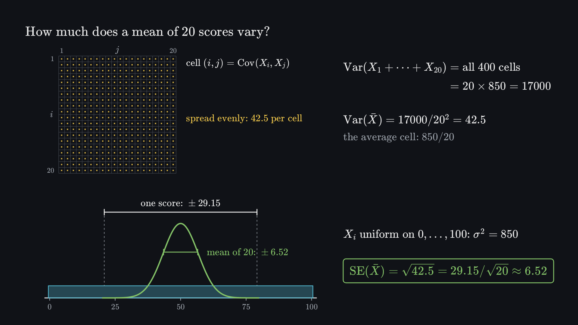
Before playing, predict: one score has SD 29.15. Is the SD of a mean of 20 scores 29.15,29.15/20 or 29.15/20?The animation’s final frame. Its numbered steps describe how the picture is built.
One score is uniform on 0,…,100, with variance σ2=850 and SD ≈29.15.
The variance of a sum of 20 scores adds up all 20×20=400 cells of a grid, where cell (i,j) is Cov(Xi,Xj).
Independent scores have zero covariance, so only the 20 diagonal cells remain, each 850: the sum has variance 20×850=17000.
The mean divides the sum by 20, so its variance is divided by 202=400: spread evenly, 42.5 per cell, so Var(Xˉ)=850/20.
So SE(Xˉ)=42.5=29.15/20≈6.52: a mean of 20 scores varies far less than one score.
3.2.5 Efficiency and consistency
Among unbiased estimators of the same target under the same model, the one with smaller sampling variance is more efficient. A noisy sample median and a sample mean may both converge to 50 for the symmetric uniform population 0,…,100. That example does not establish a universal ranking, and a median generally targets a population median rather than a mean.
Definition.θ^n is consistent for θ if, for every ε>0, P(∣θ^n−θ∣>ε)→0 as n→∞.
Read this as “the probability of an error larger than epsilon tends to zero.” It is a statement about a sequence of sampling distributions, not a promise that a realised estimate moves closer at every step.
A useful sufficient condition is vanishing mean squared error:
The inequality follows by applying Markov's inequality to squared error. Thus bias tending to zero and variance tending to zero imply consistency. This is sufficient, not a necessary characterisation of all consistent estimators.
Consistency does not require finite-sample unbiasedness. For iid draws uniformly from 0,…,1000, use their maximum to estimate the population maximum 1000. It never exceeds the target, and has positive probability of falling short for every finite n, so it is biased downwards. Yet P(maxiXi<1000)=(1000/1001)n→0. With a nested growing sample, the maximum can only stay the same or rise; it cannot bounce downwards.
Exercise. In the sample 1,2,1,3,4,4, calculate the estimated SE of the mean and explain why it is smaller than the sample SD.
Solution
We found s2=1.9, so s≈1.378 and s/6=1.9/6≈0.563. The first describes variation among six observed values; the second estimates variation of the mean across iid samples of size six. Averaging reduces independent noise. Six observations alone do not establish a normal approximation.
3.3 Sampling distributions, LLN and CLT
Concentration of averages and the shape of their remaining uncertainty
3.3.1 One sample is not a sampling distribution
A histogram of n observations depicts the observed data. A histogram of R sample means, each calculated from a separate sample of size n, depicts a simulation of the mean's sampling distribution. Keep those two counts separate: n is observations per sample; R, read “capital R,” is the number of repeated samples.
The parameter stays fixed across this thought experiment. The estimator varies because each sample changes. After one sample has been realised, its estimate is fixed too; its standard error describes the rule's uncertainty across other possible samples under the model.
For independent uniform draws on 0,…,100, individuals have SD 850≈29.15. The mean from 20 draws has SE 850/20≈6.52. Individuals can remain widely spread even when their averages are concentrated. This separation is the basis of statistical inference.
3.3.2 The law of large numbers
Weak law of large numbers. Under iid sampling with a finite mean and finite variance, the sample mean converges in probability to the population mean:
Xˉnpμ,P(∣Xˉn−μ∣>ε)→0(ε>0).
There are versions requiring weaker assumptions, but these conditions are enough for our derivation. “Weak” identifies the mode of convergence, not the practical usefulness of the result. Convergence in probability means a fixed error tolerance is increasingly unlikely to be exceeded.
Bound the chance of a large error. Chebyshev's inequality gives P(∣Xˉn−μ∣>ε)≤σ2/(nε2), which tends to zero.
The bound provides a conservative finite-sample statement when the variance is known. With variance 850, sample size 1,000, and tolerance 5, the error probability is at most 850/(1000×25)=0.034. The LLN itself is a limiting result; it does not specify that every chosen finite sample is already accurate.
A running mean may move away from its target temporarily as new observations arrive. That does not contradict convergence. Nor does more data remove selection bias: if the sample comes from the wrong distribution, the average can converge very precisely to the wrong target.
3.3.3 The central limit theorem
The LLN says the unscaled error disappears. To study the shape of the remaining error, divide it by its shrinking SE. Under iid sampling with 0<σ2<∞, the CLT states
ZnZn=σ/nXˉn−μ,dN(0,1).
The standardisation subtracts the centre and divides by the SD of the mean. Thus Zn has mean zero and variance one for every n under these assumptions, while its shape approaches a standard normal distribution.
More precisely, P(Zn≤z)→Φ(z) for each real z, where Φ is the standard normal cumulative distribution function. For sufficiently suitable large samples this motivates
Xˉn∼˙N(μ,nσ2).
The dotted relation denotes an approximation. If the parent distribution is normal, the mean is exactly normal at any sample size. Otherwise “large enough” depends on skewness, tails and rare outcomes; it has no universal threshold such as n=30.
A strongly non-normal parent
A Beta distribution with parameters 1/2,1/2 is U-shaped on (0,1), with mean 1/2 and variance 1/8. Individual samples retain that U-shaped tendency. Means from 1,000 independent samples of 50 observations can have a bell-shaped sampling histogram even though the individual measurements do not.
SE(Xˉ50)=501/8=0.05.
Standardising each mean as (Xˉ50−0.5)/0.05 allows comparison with a standard normal curve. Neither a bell-shaped simulation nor agreement with a curve proves the theorem. The assumptions and mathematical limit do that work; the simulation illustrates the distinct distributions involved.
Fixed illustration: Beta (1/2,1/2) parent, n=50. The parent has μ=0.5, SD 1/8≈0.3536; sample means have SE 0.05. The normal approximation is N(0.5,0.0025). Changing n to 200 halves the SE to 0.025, while the individual-data SD remains 0.3536.
Compare individual draws, a running mean and a histogram of repeated sample means. The seeded simulation reports the distribution, sample size and number of replications; it illustrates concentration and shape separately.Increasing sample size concentrates sample means without changing the parent distribution. Concentration of the mean and the shape of its sampling distribution are distinct questions.
3.3.4 From the theorem to an estimated SE
The CLT denominator contains σ, often unknown. If s consistently estimates σ>0, replacing the population SD by the sample SD preserves the asymptotic normal limit. This substitution is justified by the combination of consistency and Slutsky's theorem; it does not make the finite-sample distribution exactly normal.
s/nXˉn−μdN(0,1).
For iid Bernoulli data, μ=p and σ2=p(1−p). The mean is a proportion, so its estimated SE is p^(1−p^)/n. Normal approximation can be poor when expected successes np or failures n(1−p) are small. Values near the boundaries require particular care.
Variance is a nuisance parameter when our target is the mean: it is not the main object of interest, but it governs the uncertainty calculation. Estimating it matters especially with small samples. The next chapter distinguishes exact normal/known-variance inference, normal/unknown-variance inference using Student's t, and large-sample approximations.
Exercise. With the U-shaped Beta parent, find the SE for n=8 and n=128. Does reducing SE imply the individual values become normally distributed?
Solution
Use (1/8)/n: the SEs are 1/8=0.125 and 1/32=0.03125. Multiplying sample size by 16 divides SE by 4. The parent distribution remains U-shaped. The CLT concerns standardised means, and does not guarantee a good approximation at n=8.
3.4 Confidence intervals for means
Invert a sampling statement to describe uncertainty about a fixed target
3.4.1 What does confidence describe?
A point estimate gives one answer. A confidence interval adds a range constructed by a procedure whose coverage can be assessed across repeated samples. The population parameter remains fixed; the interval endpoints change when the sample changes.
Definition. A confidence procedure [L(X),U(X)] has coverage 1−α for a parameter value θ when
Pθ{L(X)≤θ≤U(X)}=1−α.
The probability is over the random sample under the model with parameter θ. For an exact procedure this statement holds as specified by its model; a large-sample procedure generally has approximate coverage.
After observing the data, the computed endpoints and the parameter are fixed. The realised interval either covers the parameter or does not. A 95% confidence interval is not a 95% posterior probability that the fixed parameter lies inside these observed endpoints. Such a probability would require a Bayesian model and prior.
If we repeatedly draw samples of size 5 from N(0,1), the known-SD intervals Xˉ±1.96/5 have approximately 95% coverage. Among 20 repetitions, the number covering is random, not guaranteed to be 19. A single observed interval cannot reveal its own coverage status when the true mean is unknown.
Before playing, predict: once one 95% interval has been computed, is there a 95% chance that it contains μ?The animation’s final frame. Its numbered steps describe how the picture is built.
Samples of n=5 from N(0,1): the mean Xˉ∼N(0,1/5) lands within 1.96/5≈0.877 of the fixed μ=0 with probability 0.95.
Each sample gives its own interval xˉ±0.877. The means −0.10 and 0.40 give intervals that contain 0.
The mean 1.00 lands outside the central 95%, so its interval [0.123,1.877] misses 0. An interval misses exactly when its mean lands outside that band.
Forty simulated samples: in this run 37 of the 40 intervals contain 0. The 95% describes the procedure over many samples; one computed interval either contains μ or does not.
Three illustrative realised means are −0.10,0.40,1.00. At n=5, known σ=1, each margin is 1.96/5≈0.877. The first two intervals contain 0; the third, [0.123,1.877], misses it. These chosen centres illustrate coverage membership, not an estimated coverage frequency.
The fixed population mean is a vertical reference. Every row is a fresh random interval. The simulation reports coverage over all replications and draws only its first rows; a short run need not equal the nominal confidence level.The vertical reference is the fixed population mean. These three chosen intervals show containment and noncontainment; long-run confidence coverage belongs to the procedure, rather than this illustrative proportion.
3.4.2 Deriving a mean interval
Start with a statement about a statistic whose distribution we know or approximate. For iid normal observations with known σ>0, Z=(Xˉ−μ)/(σ/n) is exactly standard normal. Let c=z1−α/2 be the quantile with probability α/2 above it. Symmetry puts the same probability below −c.
Central probability.P(−c≤Z≤c)=1−α.
Rescale by a positive number. Multiply the inequalities by σ/n, obtaining −cσ/n≤Xˉ−μ≤cσ/n.
Solve for the target. Subtract Xˉ, reverse the inequalities when multiplying by −1, and reorder:
e=σ/n,P(Xˉ−ce≤μ≤Xˉ+ce)=1−α,interval:Xˉ±ce.
The algebra has not made the unknown mean random. It has turned a probability statement about a random estimator into one about random endpoints containing a fixed mean. Read ± as “plus or minus”: it specifies both endpoints.
For 90%,95%,99% confidence, the standard normal critical values are approximately 1.645,1.960,2.576. Higher confidence requires a wider interval at the same SE. Width is 2cSE; quadrupling an iid sample size halves width when population variation is held fixed. Extra precision and extra confidence are different objectives.
Which critical value belongs to which model?
With an unknown SD and a suitable large sample, use Xˉ±cs/n as an approximate interval. With iid normal data and unknown SD, the exact pivot is instead
T=s/nXˉ−μ∼tn−1.
Read tn−1 as “t with n minus one degrees of freedom.” Student's t distribution has heavier tails, accounting for uncertainty in the SD estimate. Use its quantile tn−1,1−α/2 in place of c. This exact small-sample result needs normality, not just independence. For non-normal small samples, neither normal nor t calibration is automatically reliable.
3.4.3 One mean: a complete calculation
A sample has n=100, observed mean xˉ=64, and sample variance s2=8. Under the iid large-sample model, estimate the uncertainty in the population mean.
Identify the estimator.Xˉ estimates μ, with realised value 64.
Convert data spread into uncertainty of the mean.s=8; estimated SE is 8/100≈0.28284. The number 8 is a variance, not an SD.
Choose the confidence level. At 95%, use c≈1.96. Margin 1.96×0.28284≈0.55437.
Report endpoints and conditions.64±0.55437, approximately [63.446,64.554]. This is a large-sample mean interval, not a range containing 95% of individual grades.
3.4.4 Two independent means
For iid samples within each group and independence between groups, target δ=μX−μY, estimated by δ^=Xˉ−Yˉ. Subtracting changes the sign of the centre, but independent variances still add:
The estimated expression is not the unknown true variance itself. No equality of population variances is assumed in this formula.
Anchoring: state the direction before subtracting
Use the lecture's illustrative anchoring exercise: 89 students were split between a low prompt, 10, and a high prompt, 65, before giving a percentage estimate in a UN-membership question. Treat the reported summaries as teaching inputs: low group nX=43,xˉ=17.1,sX2=86; high group nY=46,yˉ=30.7,sY2=253. No current factual percentage is needed to analyse the responses.
Define the contrast. Low minus high is 17.1−30.7=−13.6 percentage points.
Estimate its sampling variance.86/43+253/46=2+5.5=7.5. SE is 7.5≈2.73861.
Construct the interval. Margin 1.967.5≈5.36768, giving [−18.968,−8.232] percentage points.
Interpret the sign. The interval is entirely negative for low minus high. Reversing the contrast gives [8.232,18.968], not the same signed interval.
Under the working model, the response difference is inconsistent with zero at the corresponding two-sided level. Random assignment can support a causal comparison of prompts, subject to implementation and response assumptions. It does not itself make these students representative of a wider population. Sampling and treatment assignment answer different questions.
Supplement: Welch's interval
For independent normal groups with unknown, possibly unequal variances, a common small-sample improvement uses Welch's approximate t calibration. Set a=sX2/nX, b=sY2/nY, and
ν=a2/(nX−1)+b2/(nY−1)(a+b)2.
Use tν,1−α/2a+b for the margin. This is an approximation with estimated degrees of freedom ν, read “nu”; it is not the exact known-variance normal case.
3.4.5 Paired means: analyse the within-pair difference
If each student takes both examinations, scores within a student may be related. Define Di=Xi−Yi for each student. Treat the n pairs as independent sampling units; there are n differences, not 2n independent observations.
DˉsD2SE(Dˉ)=Xˉ−Yˉ,=sX2+sY2−2sXY,=nsD.
Read sD as “s sub D,” the sample SD of differences. The covariance term follows by expanding Var(X−Y). Positive covariance reduces variation of differences: a student who scores high on both exams may still have a modest score difference. Marginal score SDs alone do not supply sD.
For the lecture's 71 students, the exam means are 79.6 and 81.4, variances 117 and 151, and sample correlation approximately 0.54. The supplied difference variance is 124.45, consistent with those rounded summaries. With exam 1 minus exam 2, the displayed example pairs (57.1,60.7) and (78.6,82.9) have differences −3.6 and −4.3.
Centre.dˉ=79.6−81.4=−1.8.
SE of the difference mean.124.45/71≈1.32394.
Margin and interval.1.96×1.32394≈2.59492, so the large-sample 95% interval is [−4.395,0.795].
Conclusion. The interval includes zero. These data do not establish a nonzero population mean score difference at this level. They do not prove equal means, and score differences alone cannot isolate exam difficulty from all other changes.
Exercise. Why is 117/71+151/71 inappropriate for these paired scores?
Solution
It assumes zero cross-covariance and treats the two exam samples as independent. The same students supply both measurements. The actual covariance is approximately 0.54117×151, so difference variance is 117+151−2sXY≈124.45. The appropriate SE is 124.45/71, not 268/71.
3.5 Confidence intervals for proportions
Binary means, independent contrasts and paired transitions
3.5.1 A proportion is a mean of indicators
Record Xi=1 when person i gives the response of interest and Xi=0 otherwise. Then p=P(Xi=1) is the population proportion, and p^=n−1∑iXi=k/n is the sample proportion when k successes are observed. Under iid Bernoulli sampling,
The large-sample Wald interval substitutes this estimated SE into a normal margin:
p^±cnp^(1−p^).
Read “p hat plus or minus c times its estimated standard error.” The population variance is determined by p, but p is unknown, so the CI denominator uses p^. This will differ from a null-based test denominator. Applying the generic mean formula s/n to binary data instead gives p^(1−p^)/(n−1). The customary Wald formula uses the plug-in convention shown here; these two estimated SEs are asymptotically equivalent, and neither makes the interval exact.
A survey example with bounded assumptions
The lecture reports a historical survey example with n=1502 and an approval proportion p^=0.39. Use these as classroom inputs for an iid, unweighted approximation. A published survey may have weighting and a more complex design; these summaries alone do not establish its actual design-based standard error. The rounded percentage also does not determine an exact integer success count.
Variance of an individual indicator. Plug-in value 0.39(1−0.39)=0.2379.
Variance and SE of the mean. Divide by 1502, then take the square root: 0.2379/1502≈0.0125853.
Margin.1.96×0.0125853≈0.0246671.
Interval.[0.3653,0.4147], or approximately 36.53% to 41.47%.
The margin is about 2.47percentage points, not a 2.47% relative change in approval. Keeping probability and percentage scales explicit avoids a factor-of-100 error.
Why boundaries require a better procedure
When p^=0 or 1, the Wald SE is zero. The resulting zero-width interval clearly does not express the uncertainty from a small sample. Wald endpoints can also lie outside [0,1], and coverage may be poor near boundaries. Merely clipping the endpoints does not repair the coverage calculation. The score-test inversion below produces a Wilson interval that respects the probability scale; exact binomial procedures are another option.
3.5.2 Two independent proportions
For independent groups, estimate the difference δ=pX−pY by δ^=p^X−p^Y. The two estimated variances add because the samples are independent:
There is no reason to pool the two proportions for this interval: the target permits different population proportions. The equality test later imposes a common proportion under its null and consequently uses a different denominator.
For a historical lecture knowledge question about identifying John Roberts, take the reported inputs as illustrative: 239 Republican respondents with correct-response proportion 0.47, and 238 Democrat respondents with proportion 0.31. These rounded figures describe one specific question. They do not measure general political knowledge or prove one group is “better informed” overall.
Define the contrast. Republican minus Democrat correct-response proportion: 0.47−0.31=0.16.
Unpooled SE. Compute the two variance contributions: abe=0.47(0.53)/239,=0.31(0.69)/238,=a+b≈0.044057.
Interval.0.16±1.96(0.044057), approximately [0.07365,0.24635], or 7.37 to 24.63 percentage points.
Scope. Under the working independent-sample approximation the population contrast for this response is positive. Representativeness, wording, response and design affect any broader inference.
3.5.3 Paired proportions need the joint table
With before-and-after smoking status for the same people, the two proportions are dependent. Let Bi be before status, Ai after status, with 1 denoting smoking, and define Di=Ai−Bi. Its possible values are −1 for quitting, 0 for no change, and +1 for starting. A difference of two indicators is not itself a Bernoulli indicator.
The mean difference is Dˉ=p^A−p^B. Its estimated SE is sD/n, and the large-sample interval is Dˉ±csD/n. Independence is required between people/pairs, not between measurements on the same person.
Before smoking is reported as 30% and after smoking as 25% for 100 people. Those margins give the change −0.05, but not its SE. People who quit and people who start create the variance; people unchanged in either state create zero differences.
A coherent illustrative paired table
The following table is an explicitly constructed teaching example with those same marginal counts. It is not a recovered dataset from the lecture summary.
Illustrative transitions for 100 independent people
Before status
After smoking
After not smoking
Total
Smoking
20
10
30
Not smoking
5
65
70
Total
25
75
100
Compute the difference sum. Ten quitters contribute −10, five starters +5, and 85 unchanged people zero. Therefore ∑Di=−5 and dˉ=−0.05.
Compute squared differences. Each discordant pair contributes 1, so ∑Di2=15. Use ∑(Di−dˉ)2=∑Di2−ndˉ2=15−0.25=14.75.
Estimate variance and SE.sD2=14.75/99≈0.14899; sD/100≈0.03860.
Construct the interval.−0.05±1.96(0.03860), approximately [−0.12565,0.02565].
The interval includes zero under this approximate procedure. That does not show that there is no change. It describes substantial uncertainty about the mean change. A before-and-after comparison without a suitable counterfactual also does not isolate the program's causal effect from other changes over time.
Correction to the supplied smoking summaries
The lecture lists marginal variance values 0.21 and 0.1875, correlation 0.66, and difference variance 0.4. These cannot all describe the same paired data. The covariance identity would imply
rather than 0.4. Moreover, the marginal values use the plug-in Bernoulli convention rather than the n−1 sample-variance correction. If one simply stipulates sD2=0.4, the arithmetic gives [−0.17396,0.07396]; that is a calculation conditional on an inconsistent supplied summary, not a verified interval for the original participants. The coherent table above makes every input and calculation inspectable.
3.5.4 Practise choosing the denominator
Exercise. Another table has the same 30 before smokers and 25 after smokers, but 25 smoke at both times. Find the difference variance and compare its CI with the constructed table above.
Solution
There are 5 quitters, 0 starters and 95 unchanged people. The mean remains −0.05, but ∑Di2=5. Thus sD2=(5−100(0.05)2)/99=4.75/99≈0.04798, SE 0.04798/100≈0.02190, and the approximate Wald CI is [−0.09293,−0.00707]. Same marginal change, different uncertainty. With only five discordant pairs the normal approximation is fragile; an exact paired-binomial test is preferable to treating this result as definitive.
Exercise. Why is the single-proportion SE based on p^(1−p^), but the paired-change SE cannot be found from that expression applied to −0.05?
Solution
A Bernoulli variable takes values 0,1 and has a probability mean between zero and one. A paired difference takes −1,0,1, and its mean can be negative. Its variance depends on the proportion of discordant pairs, not just its mean. Compute sD2 from the differences or from the full paired table.
3.6 Hypothesis testing and evidence
Calibrate a decision under a null model without reversing its probability
In this chapter
By the end you should be able to:
State null and alternative hypotheses about a population parameter, with the direction fixed in advance.
Explain Type I and Type II errors, the significance level and power.
Calculate a large-sample z statistic and its p-value, and reach a decision at a stated level.
Interpret a p-value correctly and report a test result in context.
A hypothesis concerns a population parameter, not the already observed statistic. “The population mean grade is 66” is a testable claim H0:μ=66. “The observed sample mean is 64” is a description of data, not an uncertain population hypothesis.
For a two-sided test of a specified value, write
H0:θ=θ0,H1:θ=θ0.
Here H0 is the null hypothesis, H1 the alternative, and θ0 the numerical value hypothesised. A null of equal average A-level scores for two demographic groups has θ=μX−μY, θ0=0. Equal outcome proportions across two groups similarly uses θ=pX−pY. A hypothetical COVID-19 mortality comparison must first define the population, denominator and time period consistently; naming two groups alone does not define comparable probabilities.
A one-sided alternative, such as θ>θ0, asks a different question and puts rejection probability in one tail. Its null includes values θ≤θ0; calibration commonly uses the boundary θ0. Choose the direction before examining the result, rather than selecting whichever tail looks favourable.
3.6.2 Error rates describe repeated decisions
Truth and decision are distinct dimensions
Population truth
Fail to reject
Reject
H0 true
Correct decision
Type I error
H0 false
Type II error
Correct detection
A Type I error rejects a true null. A Type II error fails to reject a false null. The significance level α controls the rejection probability under the null:
P(reject H0∣H0 true)≤α.
Think first. A test at the 5% level rejects the null. Is there now only a 5% chance that the null is true?
Answer
No. The level bounds P(reject H0∣H0 true): how often the procedure rejects when the null is true. The question asks for P(H0 true∣reject), which reverses the conditioning, as in Bayes’ rule (1.3). That reversed probability also depends on how often the hypotheses being tested are true and on the test’s power. A 5% level therefore does not mean an observed rejection has a 5% chance of being wrong.
At a specified alternative value θ, the Type II probability is β(θ), read “beta at theta,” and power is 1−β(θ): the probability of rejecting there. Power depends on effect size, variation, sample size and the rejection rule. Lowering α with everything else fixed usually makes rejection harder and reduces power.
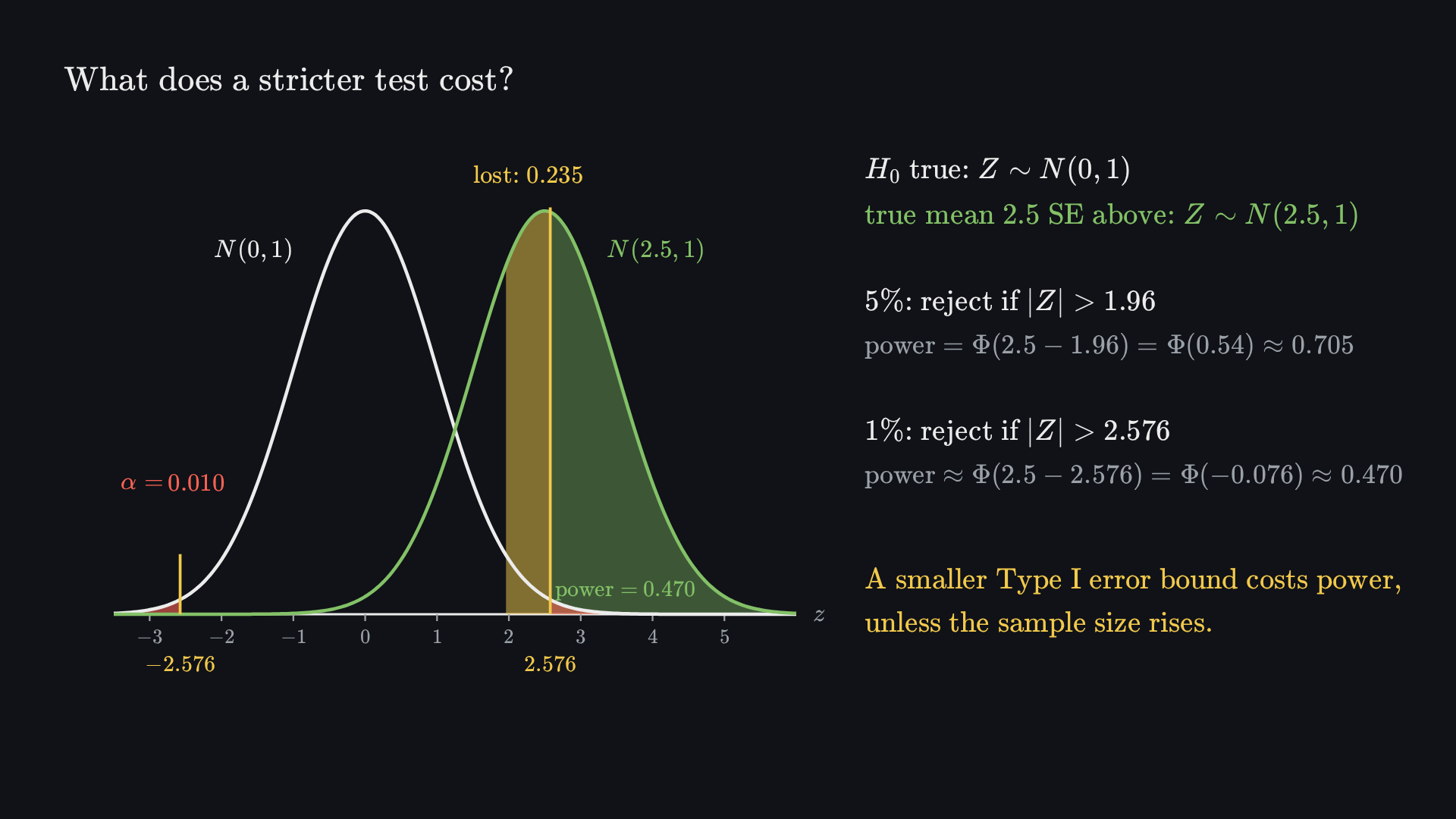
Before playing, predict: if a two-sided test at 5% is made stricter, at 1%, what happens to its chance of detecting a real effect?The animation’s final frame. Its numbered steps describe how the picture is built.
If H0 is true, Z∼N(0,1). If the true mean lies 2.5 standard errors above the null value, Z∼N(2.5,1).
At 5%, reject when ∣Z∣>1.96: the red tails of the null curve have area 0.05. The power is the green area of the true curve beyond the cutoffs, Φ(0.54)≈0.705.
Lower the level to 1%: the cutoffs move out to ±2.576. The red tails shrink to 0.01, and the power falls to Φ(−0.076)≈0.470.
The yellow strip between 1.96 and 2.576 is the power given up, about 0.235. A smaller Type I error bound costs power unless the sample size rises.
The trial analogy helps explain “fail to reject” versus “prove true”: an acquittal does not establish innocence. But the analogy does not make Type I errors universally worse. Error costs depend on the application, and statistical thresholds are not legal standards.
3.6.3 Build and calibrate the statistic
The test compares the observed distance from the null with the distance expected from sampling variation under that null. A common large-sample form is
Z=SE0(θ^)θ^−θ0.
The subscript 0 stresses null calibration. The numerator is an effect in its original units; division expresses it in SE units. Under the assumptions of the relevant procedure, Z is approximately N(0,1) under H0. A statistic far from zero is unusual under the whole null model, including its sampling and variance assumptions.
State the estimand and hypotheses. Fix the subtraction direction and whether the alternative is one- or two-sided.
Construct the statistic. Use the SE appropriate to the design and the null.
State the null distribution and assumptions. Distinguish exact calibration from an approximation.
Choose the level. For a two-sided normal test, reject when ∣Z∣>z1−α/2; each tail has probability α/2.
Report the decision in context. Give the estimated effect, uncertainty and evidence. Use “fail to reject,” not “accept” or “prove equal.”
Two-sided normal critical values are 1.645 at 10%, 1.960 at 5%, and 2.576 at 1%. For a pre-specified upper-sided 5% test, the critical value is 1.645. The same numerical cutoff can therefore have different meanings depending on the tail rule.
3.6.4 A p-value is a null-model tail area
Definition. A p-value is the probability, calculated under the null model, of a test statistic at least as extreme as the observed statistic according to the pre-specified alternative.
For a two-sided standard normal test with observed value zobs,
pval=2{1−Φ(∣zobs∣)}.
Here pval labels a p-value; it is unrelated to a population proportion p. For an upper-sided test use 1−Φ(zobs); for a lower-sided test use Φ(zobs). A small p-value indicates that the statistic is unusual under the null model.
Common mistake
Reading a p-value as the probability that the null is true. The p-value is calculated assuming the null model, so it cannot also be the probability of that model. Nor is it the probability that chance “caused” the observation, or that a future experiment will reproduce the result.
For a continuous calibrated statistic, the rule pval<α matches the critical-value rule. Discrete exact tests can have attainable rejection probabilities below the nominal level; precise equality conventions can matter at a boundary. We use non-rejection at equality in the displayed continuous rules.
Fixed two-sided normal tails at an observed z=2
Fixed normal illustration: observed z=2. A two-sided p-value is 2(1−Φ(2))≈0.04550; an upper-sided p-value is 1−Φ(2)≈0.02275; a lower-sided p-value is Φ(2)≈0.97725. At 5%, the first two reject their respective nulls; the lower-sided test does not.
The shaded region represents outcomes at least as extreme under the selected alternative. Changing the alternative changes the tail area; the observed statistic alone does not define a p-value.For the two-sided alternative, both tails beyond −2 and 2 count as at least as extreme. The drawing stops at ±4; the numerical p-value includes the more distant tails as well. A one-sided alternative selects only its specified tail.
3.6.5One test from start to finish
Return to the grade sample from 3.4: n=100 scripts, sample mean xˉ=64 and sample variance s2=8. Suppose a department claims that the population mean grade is still 64.5. Follow the five steps of 3.6.3.
Worked example
State the estimand and hypotheses. The estimand is the population mean grade μ. Before looking at the result, choose a two-sided alternative: H0:μ=64.5, H1:μ=64.5.
Construct the statistic. The estimated SE is 8/100≈0.2828, so z=0.282864−64.5≈−1.77. The sample mean lies 1.77 standard errors below the claimed value.
State the null distribution and assumptions. With iid sampling and n=100, Z is approximately N(0,1) under H0. This is a large-sample approximation, not an exact result.
Choose the level and compare. At α=0.05 the two-sided critical value is 1.960, and ∣z∣=1.77<1.960. Equivalently, pval=2{1−Φ(1.77)}≈0.077>0.05.
Report the decision in context. We fail to reject H0 at 5%. The sample mean is below 64.5, but a difference at least this large, in either direction, would occur in about 8% of samples if the claim were true. Report the estimate, the 95% interval [63.45,64.55] and pval≈0.077, not only the decision.
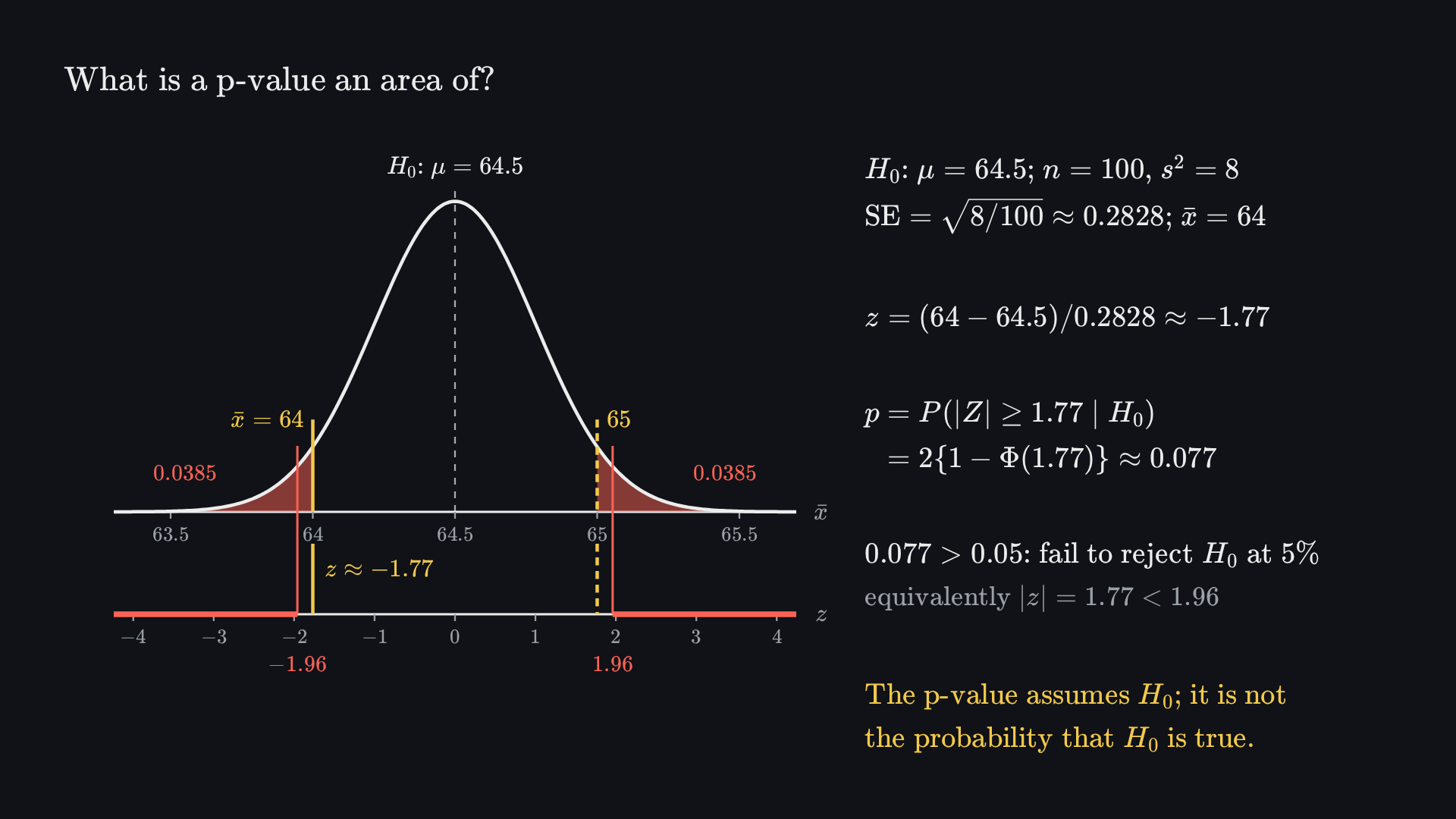
Before playing, predict: the sample mean lies 1.77 standard errors below the claimed 64.5. Is that significant in a two-sided test at 5%?The animation’s final frame. Its numbered steps describe how the picture is built.
If H0:μ=64.5 were true, means of 100 scores would vary around 64.5 with SE=8/100≈0.2828. The observed mean is 64.
Standardise: z=(64−64.5)/0.2828≈−1.77. The observed mean lies 1.77 standard errors below the claim.
Two-sided, a result at least as extreme lies 1.77 or more standard errors away in either direction: p=2{1−Φ(1.77)}≈0.077.
At 5% the cutoffs are ±1.96 and 0.077>0.05, so we fail to reject H0; at 10%, with cutoff 1.645, we would reject. The p-value is computed assuming H0, so it is not the probability that H0 is true.
Two comparisons show what the decision depends on. At α=0.10 the critical value is 1.645<1.77, so the same data would reject: the level is part of the rule and must be fixed in advance. In 3.7.1 the same sample rejects the claim μ=65, which lies 3.54 standard errors from xˉ. The interval [63.45,64.55] contains 64.5 but not 65; 3.8 shows why intervals and tests agree in this way.
Common mistake
“We failed to reject, so μ=64.5.” Non-rejection says the data are compatible with 64.5 at this level. They are also compatible with other values inside the interval, such as 64.0 or 64.3. Showing that a parameter is close to a value needs a pre-specified tolerance and a procedure designed for that question (3.6.6).
3.6.6 Significance, relevance and replication
A small effect can be statistically significant in a large precise sample; a consequential effect can remain uncertain in a small noisy sample. Report effect size and an interval alongside the test. Failure to reject zero is not an equivalence result. To establish practical equivalence, pre-specify a meaningful tolerance and use a procedure designed for that question.
Repeated testing also changes the chance of a false finding. Under 20 independent true-null tests at 5%, the probability of at least one rejection is 1−0.9520≈0.642. Without independence, the union bound still gives an upper bound of 20×0.05, capped at 1. Choosing analyses after observing their p-values can therefore invalidate the promised error rate.
Replication examples and what their percentages mean
The 2015 Open Science Collaboration study examined 100 studies from three psychology journals. It reported 36% statistically significant replications and 39% subjectively judged replications. These are different criteria; neither is a universal replication probability.
The 2016 economics replication study found a significant effect in the original direction in 11 of 18 laboratory studies, approximately 61%, with other criteria giving other rates. A subsequent proposal advocated a 0.005 threshold for claims of new discoveries. That proposal is not a theorem making one cutoff universally appropriate. Design, power, multiplicity, effect estimation and transparent analysis remain essential.
3.6.7Exercises
Try each question before opening any help. A hint points to the first step, the answer lets you check your result, and the full solution shows every step.
Exercise 1. A two-sided test gives z=1.5 and p-value approximately 0.134. At 5%, can we say the null has probability 0.866 or that the effect is zero?
Hint
Under which model is a p-value calculated? What does non-rejection allow you to say?
Answer
No to both. We fail to reject at 5%, but that neither gives the null a probability nor shows that the effect is zero.
Full solution
No to both. The p-value is a probability of sufficiently extreme statistics under the null model, not a probability assigned to the hypothesis. Since 0.134>0.05, we fail to reject at the chosen level. The estimate and interval can still permit substantively important nonzero effects.
Exercise 2. A random sample of n=64 scripts has mean xˉ=67.8 and sample standard deviation s=8. (a) Test H0:μ=66 against H1:μ=66 at 5%. (b) What would the p-value be if the upper-sided alternative μ>66 had been chosen before seeing the data? (c) Why may the upper-sided test not be chosen after seeing xˉ=67.8?
Hint
Start with SE=s/n. A two-sided p-value counts both tails; an upper-sided p-value counts one.
Answer
(a) z=1.8 and pval≈0.072: fail to reject at 5%. (b) pval≈0.036. (c) Choosing the tail after seeing the data makes the Type I error rate 10%, not 5%.
Full solution
Standard error.SE=8/64=1.
Statistic.z=(67.8−66)/1=1.8.
Two-sided p-value.2{1−Φ(1.8)}≈2(0.036)=0.072>0.05, so we fail to reject at 5%. Equivalently, 1.8<1.960.
Upper-sided p-value.1−Φ(1.8)≈0.036<0.05. A pre-specified upper-sided test rejects, because its critical value is 1.645.
Why the tail must come first. If the tail is chosen to match the sign of z, the procedure rejects whenever ∣Z∣>1.645. Under the null that happens with probability 2(0.05)=0.10, double the stated level.
Exercise 3. A study keeps its sample size fixed but lowers the level of a two-sided normal test from 5% to 1%. Suppose the true mean lies 2.5 standard errors above the null value, so that Z is approximately N(2.5,1). Find the power at each level and explain the trade-off.
Hint
Power is the probability of rejection. Use the critical values 1.960 and 2.576, and find P(Z>c) when Z∼N(2.5,1); the opposite tail is negligible here.
Answer
Power is about 0.705 at 5% and 0.470 at 1%. The smaller Type I error bound costs power unless the sample size rises.
Full solution
Standardise under the alternative. If Z∼N(2.5,1), then P(Z>c)=1−Φ(c−2.5)=Φ(2.5−c).
Level 5%. With c=1.960, power ≈Φ(0.54)≈0.705. The lower tail adds Φ(−4.46), which is below 0.00001.
Level 1%. With c=2.576, power ≈Φ(−0.076)≈0.470.
Trade-off. The Type I error bound falls from 0.05 to 0.01, while the probability of detecting this effect falls from about 0.71 to 0.47. A stricter level can be worth it when false positives are costly. Keeping the power requires a larger sample, which shrinks the SE and moves the true mean further from the null value in SE units.
Exercise 4. A study tests 10 independent outcomes, and every null hypothesis is true. Each test uses α=0.05. (a) Find the probability of at least one rejection. (b) Which per-test level α∗, read “alpha star”, keeps the union bound on that probability at 0.05, with or without independence?
Hint
For (a), use the complement: no rejection at all. For (b), the union bound adds the ten rejection probabilities.
Answer
(a) 1−0.9510≈0.401. (b) α∗=0.05/10=0.005.
Full solution
Complement. With independent tests, P(no rejection)=0.9510≈0.599.
At least one rejection.1−0.9510≈0.401. With ten true nulls, at least one false finding has about a 40% chance of appearing.
Union bound. For any dependence between the tests, P(at least one rejection)≤10α∗. Setting 10α∗=0.05 gives α∗=0.005.
Check under independence.1−0.99510≈0.049≤0.05. This adjustment is the Bonferroni correction. It controls the chance of any false rejection, at a cost in power for each test.
3.6.8Review
Check yourself
Choose an answer to see why it is right or wrong. Nothing is recorded.
Key ideas
A hypothesis is a claim about a population parameter. Fix H0, H1 and the direction before looking at the result.
The level α bounds the probability of rejecting a true null. It is not the probability that a rejection is wrong.
A test statistic measures the distance from the null value in standard errors: Z=(θ^−θ0)/SE0.
A p-value is a tail area under the null model. Reject when pval<α; never read it as the probability that H0 is true.
“Fail to reject” is not “accept”. Report the estimate and an interval with the decision.
Power rises with the effect size and the sample size, and falls as α falls. Many tests, or tests chosen after seeing the data, inflate false findings.
3.7 Tests for means and proportions
Choose the sampling unit and calibrate the correct denominator
3.7.1 Three mean tests, one pattern
For means, the estimated SE typically does not depend on the hypothesised mean. Use the same independent or paired structure as in the matching confidence interval. The large-sample statistics are
The numerator subtracts the hypothesised numerical differenceδ0, not the unknown true population difference. Under a null of equality it is zero. These normal references are approximate for generic iid data. The exact normal-population one-sample or paired procedure uses Student's t; independent unequal-variance groups can use Welch's approximation.
Single mean: test the claim μ=65
Hypotheses.H0:μ=65, H1:μ=65.
Inputs and statistic. With n=100,xˉ=64,s2=8, SE is 8/100=0.28284, and z=(64−65)/0.28284≈−3.5355.
Calibration. Under the iid large-sample model, use standard normal tails. The two-sided p-value is approximately 0.000407.
Decision. At α=0.05, ∣z∣>1.96, so reject. The observed mean is lower than the claim; the matching interval [63.446,64.554] excludes 65.
Independent means: the anchoring contrast
Hypotheses and direction. Low minus high, H0:μX−μY=0 versus a nonzero difference.
Statistic. The estimate is −13.6, SE is 86/43+253/46=7.5, so z≈−4.9660.
Calibration and decision. Approximate two-sided normal p-value 6.83×10⁻⁷. Reject at 5%; the matching interval [−18.968,−8.232] excludes zero.
Scope. This is evidence about the response contrast under the stated group model. A p-value does not demonstrate accurate answers to the factual question or population representativeness.
Paired means: the examination contrast
Sampling unit. Each of 71 students contributes one exam-1-minus-exam-2 difference.
Hypotheses.H0:μD=0, H1:μD=0.
Statistic.dˉ=−1.8, SE 124.45/71≈1.32394, so z≈−1.3596.
Decision. Approximate p-value 0.1740. Since ∣z∣<1.96, fail to reject at 5%. The matching interval includes zero, but does not establish equality or identify why scores differ.
3.7.2 One proportion: use the null variance
Under H0:p=p0, the Bernoulli variance is specified by the null, so the null SE is p0(1−p0)/n. The large-sample score statistic is
Z=p0(1−p0)/np^−p0.
This denominator differs from the Wald CI's estimated denominator. It gives the sampling scale of the proportion if the claim is true. Normal approximation requires adequate expected successes np0 and failures n(1−p0). At p0=0 or 1, the null distribution is degenerate and this quotient is not defined; use the model directly.
Survey hypotheses. Test an evenly split population: H0:p=0.5, H1:p=0.5.
Null SE. With lecture inputs n=1502,p^=0.39, use 0.5(0.5)/1502≈0.01290135.
Statistic.z=(0.39−0.5)/0.01290135≈−8.5262.
Decision and assumptions. The normal-reference two-sided p-value is approximately 1.51×10⁻¹⁷, so reject at 5% under this iid classroom approximation. This is not a reconstruction of an exact survey-design analysis from rounded percentages.
Supplement: an exact binomial reference
If K is an integer success count from iid Bernoulli trials, then under the null K∼Binomial(n,p0). An exact test sums probabilities of outcomes at least as extreme according to a specified ordering. Multiple two-sided conventions exist, so state the rule. A rounded reported percentage may not identify K; do not invent a success count to claim an exact result.
3.7.3 Equality of independent proportions: pool under the null
For H0:pX=pY, the null imposes a common unknown value π, read “pi.” Pool the observed successes to estimate it:
The pooled proportion is a sample-size-weighted mean, not generally the simple average of the two percentages. For exact counts it is total successes divided by total observations. Independent sampling permits the variance terms to add. Pooling is justified here by equality under the null; it is not a valid general recipe for H0:pX−pY=δ0=0.
Hypotheses. For the illustrative knowledge-question inputs, test H0:pX−pY=0 against a nonzero contrast.
Pool.π^=(239×0.47+238×0.31)/477≈0.390168.
Null SE and numerator. SE ≈0.0446686. The numerator is 0.47−0.31=0.16, not 0.47−0.39.
Test.z=0.16/0.0446686≈3.58193, with approximate two-sided p-value 0.000341. Reject equality at 5% under the working model.
The independent-proportion confidence interval used an unpooled SE and answers an estimation question without imposing equality. These two conventional procedures may agree on many examples but are not exact inverses of one another.
3.7.4 Paired proportions: test changes within people
For the coherent illustrative smoking table, keep D=A−B. Test H0:E[D]=0 against a nonzero mean change. The paired Wald statistic uses the observed difference variance:
Z=sD/nDˉ.
Inputs.n=100,dˉ=−0.05,sD2=14.75/99.
Statistic.z=−0.05/0.0385992≈−1.29536.
Normal-reference decision. Approximate two-sided p-value 0.1952, so fail to reject at 5%. The matching paired Wald CI includes zero.
Limits. Discordant pairs number only 15; the normal reference deserves caution. A before-and-after null of no marginal change is not the same as a demonstrated absence of causal program effects.
If one instead stipulates the inconsistent lecture summary's sD2=0.4, the arithmetic gives z=−0.79057 for after minus before, and also fails to reject. The sign reverses for before minus after, but the two-sided decision is unchanged. The stipulated variance cannot repair the contradictory paired summaries.
Supplement: why the exact McNemar test uses only discordant pairs
Under equality of the two marginal smoking probabilities, the probability of quitting equals the probability of starting. Conditional on being discordant, either direction therefore has probability 1/2. For independent pairs, conditional on m discordant pairs, the number in one direction is Binomial(m,1/2).
Our table has m=15, with 5 starters and 10 quitters. The two-sided equal-tail exact p-value is
2k=0∑5(k15)2−15=0.3017578.
This exact conditional test also fails to reject at 5%. Its p-value differs from the Wald normal approximation because the reference distribution and statistic differ. Always match an interval to the test actually chosen.
Exercise. A researcher pools the before and after percentages and uses the independent-proportions SE. What assumption has been inserted?
Solution
The calculation has treated measurements on the same person as independent groups, omitting their covariance. For paired data the variance of the difference depends on transitions. Use within-pair differences or a paired binary procedure, with independence between people as the relevant sampling assumption.
3.8 Matching confidence intervals and tests
An interval is the set of null values not rejected by a specified procedure
3.8.1 Invert the same test
Imagine repeating a test on the same observed data, but changing the proposed population value θ0. Some values are too far from the estimate and rejected; others are not rejected. The set of values retained by a level-α test is its matching (1−α) confidence set.
This connection also explains coverage. For the true parameter θ, exclusion from the inverted set happens exactly when its own null is rejected. If the test's Type I probability is at most α, the inverted set contains θ with probability at least 1−α. Approximate tests yield approximate coverage; the inversion alone does not correct a poorly calibrated model.
A fixed estimated SE gives a symmetric interval
Suppose the test uses the same positive estimated SE e for every proposed mean. At a two-sided normal level, non-rejection means
Critical-value rule.(θ^−θ0)/e≤c.
Multiply by e>0.−ce≤θ^−θ0≤ce.
Solve for the proposed value.θ^−ce≤θ0≤θ^+ce.
The retained nulls form [θ^−ce,θ^+ce]. This is exactly the algebra behind the mean interval. It applies equally to an independent difference or a paired difference when the same SE and critical-value method are used.
For the single-mean example, the 95% large-sample interval is [63.446,64.554]. A proposed μ0=64.2 lies inside and is not rejected by the matching 5% test; 65 lies outside and is rejected. If μ0=xˉ−1.97e, the statistic is +1.97, because subtracting a value below the estimate gives a positive numerator. Only the absolute magnitude controls a two-sided decision.
Fixed example: xˉ=64, estimated SE e=8/100=0.282843, 95% normal interval [63.446,64.554]. Testing μ0=65 gives z=−3.5355, two-sided p-value 0.000407: reject. Testing μ0=64.2 gives z≈−0.7071, p-value 0.4795: do not reject. Each decision agrees with interval membership because the methods are matched.
Vary the proposed null on fixed data. For a mean, the fixed SE produces a symmetric interval. For a proportion, the null-dependent score SE produces a Wilson interval instead of the Wald interval.The two proposed means use the same observed data, SE and confidence interval. Their test decisions agree with interval membership because each test is the one inverted to obtain that interval.
3.8.2 A null-dependent SE changes the interval
The one-proportion score test uses p0(1−p0) in its denominator. When we vary the proposed p0, we vary its SE too. We therefore cannot invert this test merely by adding and subtracting a margin calculated at p^.
The following derivation is a supplement to the large-sample Wald approach. The score non-rejection inequality, for 0<p0<1, is
These endpoints form the Wilson interval, the inversion of this score test. Unlike the Wald interval, its centre is pulled toward 1/2, and the margin remains positive when no successes or no failures are observed. Boundary points are included using the underlying degenerate-null model.
For a supplementary example of 0 successes in 10 iid trials, the 95% Wald interval is [0,0], while the Wilson interval is approximately [0,0.2775]. Neither implies that a zero observed count proves the population probability zero. Wilson coverage is approximate, not exact at every finite-sample probability.
Similarly, the usual independent-proportion equality test pools under the null, while its common Wald difference CI does not. Do not claim exact duality between those mismatched procedures. A test obtained by inverting a specified difference interval will use that interval's own calibration; a score-based difference interval requires an appropriate constrained calculation.
3.8.3 What must match?
Test–interval duality requires the same data, target, sampling assumptions, SE construction, reference distribution, tail rule and level. A two-sided 5% test matches a two-sided 95% confidence set from that test. A one-sided 5% test instead matches the appropriate one-sided 95% bound. A t test matches a t interval with the same degrees of freedom, rather than a normal interval merely sharing a label.
Confidence intervals retain values not rejected by a procedure; they do not establish every retained value as equally plausible or true. Their width makes the remaining uncertainty visible. If zero lies inside a difference interval, examine which nonzero differences also remain compatible with the data before declaring an effect absent.
Exercise. A 95% interval computed as θ^±1.96e contains θ0. Must every two-sided test of that value at 5% fail to reject?
Solution
Only the matching test with statistic (θ^−θ0)/e and the same normal critical value must fail to reject. A procedure using a null-dependent variance, another distribution, another design, or another target need not agree. Duality connects one specified test to its own inverted confidence set.
Exercise. An interval for μX−μY is [−4.395,0.795]. Give the interval for μY−μX and the corresponding decision for equality.
Solution
Negate and reorder the endpoints, giving [−0.795,4.395]. Both include zero, so both matching two-sided equality tests fail to reject. The estimate's sign reverses; its SE, absolute test statistic and two-sided p-value remain unchanged.
![Final frame: the sampling distribution of the mean, N(0, 1/5), with its central 95% between −0.877 and 0.877 shaded and its two 2.5% tails in red; dashed lines continue the band’s edges down the page, and a fixed dashed line marks μ = 0. Below, 40 simulated intervals x̄ ± 0.877: those whose mean lies inside the band cross the μ line (green); 3 whose mean lies outside miss it (red). Beside it: n = 5 from N(0, 1), X̄ ~ N(0, 1/5); 1.96/√5 ≈ 0.877, so P(|X̄ − μ| ≤ 0.877) = 0.95; each sample gives the interval x̄ ± 0.877; 1.00 ± 0.877 = [0.123, 1.877] misses 0; a miss happens exactly when x̄ lands outside the 95% band; this run: 37 of 40 contain 0; 95% describes the procedure over many samples, and one computed interval either contains μ or not.](media/coverage-end.png?v=3306c2f419)