4.1.1 Time order changes the question

First record the frequency, units and definition. Quarterly nominal income in pounds is not quarterly real income; a stock measured at month-end is not a monthly flow. A missing month is not a zero. When observations are equally spaced, a one-period lag has a stable duration. With irregular dates, a lag of one row can mean different elapsed times, so models developed for fixed intervals require care.

Time ordering makes dependence a central possibility, but it does not guarantee it. Independent monthly draws are a time series. Cross-sectional observations can also be dependent through households, schools or markets. Independence must come from a sampling design or a model, rather than from the shape of a spreadsheet.

For forecasting, keep the information set explicit. At date $t$, an observation at $t+1$ is unavailable. A model that uses a future value to predict the past can fit well while failing as a usable forecast. Later chapters will distinguish an explanatory association from a causal effect; chronology alone establishes neither.

4.1.2 Read a plot in layers

Begin with a plot against date, then ask separate questions about the centre, spread and repeated patterns. A trend is a sustained change in level over the window. A linear trend adds roughly the same amount each period; an exponential trend multiplies by roughly the same factor. This distinction matters because equal absolute changes and equal percentage changes answer different economic questions.

Seasonality repeats at a known calendar frequency: four quarters or twelve months, for example. A cycle has rises and falls whose timing need not repeat at a fixed period. A business-cycle description may distinguish expansion, peak, contraction and trough without treating each cycle as an identical sine wave. A structural break changes a model feature, such as its mean, slope or volatility, at a date. A break can be visible after the event without being predictable beforehand.

A rising spread can accompany a rising level. If a series doubles while its typical deviations also double, variability may be proportional to level. That motivates a log scale. It does not show that the underlying uncertainty has disappeared. Equally, a flat-looking graph can conceal dependence or changing distributions. Plot appearance suggests questions; the model and its assumptions supply the answers.

A useful descriptive decomposition is $X_t=m_t+s_t+U_t$, where $m_t$ represents a trend, $s_t$ a seasonal component, and $U_t$ the remaining component. This is an additive model, not a universal identity with uniquely identified pieces. A multiplicative alternative, $X_t=M_tS_tV_t$, becomes additive after logging positive factors. The decomposition should reflect the units and the question, rather than follow the plot mechanically.

4.1.3 Dependence across dates

The population autocorrelation concerns the probability model. A sample autocorrelation estimates a feature from one realised sequence. At lag $h$, there are only $T-h$ available pairs, so long-lag estimates use fewer comparisons. At lag zero, a variable correlates perfectly with itself if its variance is positive. For a constant series the correlation denominator is zero and the coefficient is undefined.

Different correlogram shapes suggest different questions. Slow decay can accompany persistent dynamics or a nonstationary level. Peaks at lags four, eight and twelve can suggest quarterly seasonality. Small sample correlations may be compatible with white noise, but they do not prove independence or rule out nonlinear predictability. A trend can induce a persuasive correlogram even when the remaining shocks are independent.

4.2.1 Move through the index carefully

With $T$ observations, a first difference provides $T-1$ values. A four-period difference provides $T-4$. These losses are part of the definition, not a software malfunction. Never replace an unavailable lag with zero unless zero is an actual observed value justified by the model.

Two superficially similar expressions have different meanings. A quarterly year-on-year, or seasonal, difference is $\Delta_4X_t=X_t-X_{t-4}=(1-L^4)X_t$. The fourth iterated difference instead applies the first-difference operation four times:

The first compares matching quarters; the second uses five consecutive observations with binomial weights. Their notation should not be interchanged. For a perfectly repeating quarterly component $s_t=s_{t-4}$, seasonal differencing cancels that component. It may leave a trend or serially correlated shocks.

4.2.2 Growth factors compound

For a positive level series, define the one-period proportional growth rate as $g_t=X_t/X_{t-1}-1$. Then $1+g_t$ is the growth factor and $X_t=(1+g_t)X_{t-1}$. A rate of $0.05$ means $5\%$, whereas the factor is $1.05$. A nonzero denominator is necessary for the ratio; conventional compounded-growth interpretations use positive levels.

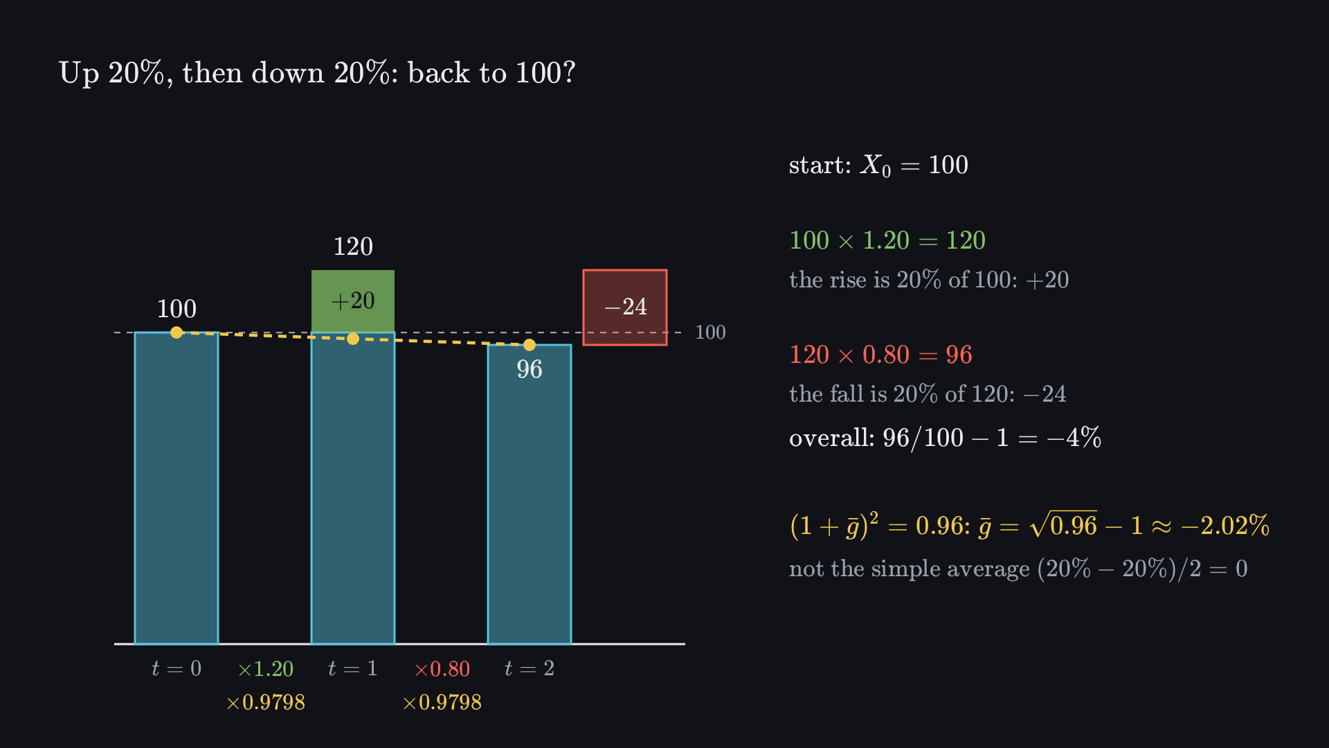
Worked question. A hypothetical index starts at $100$, rises by $20\%$, then falls by $20\%$. Has it returned to its starting value?

1. First growth factor. $100(1.20)=120$.
2. Second growth factor. $120(0.80)=96$. The decrease is applied to the new, larger base.
3. Overall change. $96/100-1=-0.04$, a $4\%$ decline. Adding the two percentages would miss the changing denominator.

To find a constant rate that produces the same endpoint over $h$ periods, ask which factor compounded $h$ times equals the observed ratio. This gives the geometric average growth rate:

Equivalently, $1+\bar g$ is the geometric mean of the intervening growth factors. In the example, $\bar g=\sqrt{0.96}-1\approx-0.02020$, or about $-2.02\%$ per period. The arithmetic average of the two rates is zero; it is not the equivalent compounded rate. Geometric averaging answers an endpoint-compounding question, while arithmetic averaging answers a different question about average one-period rates.

1. An index starts at $100\text{.}$
2. It rises by $20\%\text{:}$ $100\times1.20=120\text{.}$ The rise is $20\%$ of $100\text{,}$ so $+20\text{.}$
3. It falls by $20\%\text{:}$ $120\times0.80=96\text{.}$ The fall is $20\%$ of the larger base $120\text{,}$ so $-24\text{.}$ Overall, $96/100-1=-4\%\text{.}$
4. A steady rate with the same endpoint compounds twice to $0.96\text{:}$ $\bar g=\sqrt{0.96}-1\approx-2.02\%$ per period, not the simple average of the two rates, $0\text{.}$

The observation interval matters. If a quarterly series rises by $2\%$ each quarter, its compounded annual growth rate is $(1.02)^4-1\approx8.243\%$. Multiplying by four gives an approximation, $8\%$, rather than the exact compound result. Conversely, an annual rate should be converted by taking the appropriate root if a constant quarterly equivalent is intended.

4.2.3 Logs connect levels, ratios and differences

Log changes add through time because logarithms turn products into sums. Across $h$ periods, $\sum r_j=\log(X_t/X_{t-h})$. Dividing that total by $h$ gives the average log growth, and exponentiating it gives the geometric average factor. This is the algebra behind the preceding growth calculation.

Logs can stabilise proportional variability, but a log transformation does not generally remove a trend or a stochastic trend. A positive exponential trend becomes linear and still changes its mean with time. Logging zero or negative data is undefined. Adding an arbitrary constant makes the logarithm computable but changes ratios and the economic interpretation; it should not be treated as an innocent repair. A square-root transformation can be useful for some nonnegative series, but suitability must come from the data-generating model.

4.3.1 Deterministic and stochastic descriptions

A deterministic sequence is specified by a rule and its parameters. For $X_t=\beta_0+\beta_1t$, knowing the two coefficients determines every value. With $\beta_0=0$ and $\beta_1=1/2$, the sequence is $0,0.5,1,1.5,\ldots$. A deterministic seasonal rule such as $\sin(\pi t/2)$ repeats every four integer periods. Knowing its phase matters: the calendar position determines where the sequence is in its cycle.

Deterministic does not mean simple or periodic. In continuous time, $\sin(\pi t)+\sin(\sqrt{2}\pi t)$ combines incommensurate frequencies and has no common positive period. If sampled only at integer dates, the first sine is zero, so the sampled sequence differs from the continuous curve. Always distinguish a mathematical time domain from the frequency at which observations are collected.

A stochastic model specifies a probability law rather than one unique realised future. It can have a completely explicit formula. For example, $X_t=0.7X_{t-1}+\varepsilon_t$ is a formula whose future values depend on random innovations. “Random” does not mean that the model is unwritable; it means that the rule describes distributions of possible paths.

To combine a deterministic and a random component, write $X_t=m_t+\sigma_tZ_t$, with independent standard-normal $Z_t$. Then $E[X_t]=m_t$ and $\operatorname{Var}(X_t)=\sigma_t^2$. A changing $m_t$ produces a changing mean; a changing $\sigma_t$ produces changing variability. The draws can remain independent across dates in both examples. These are sums or scaled components; a convolution is a different mathematical operation and is not a synonym for combining curves.

4.3.2 What must stay unchanged?

Stationarity allows us to regard different segments of time as governed by the same relevant probabilistic structure. It permits dependence across dates while restricting how that dependence changes with the calendar. Relative positions may matter; absolute date does not.

Strict stationarity. Every finite collection of observations has the same joint distribution after a common time shift: $(X_{t_1},\ldots,X_{t_k})$ and $(X_{t_1+a},\ldots,X_{t_k+a})$ have the same distribution whenever those indices are in the process’s domain.

“Every joint distribution” is stronger than a claim about each individual date. It includes how neighbouring values co-vary and how larger collections behave. Identically distributed independent draws are strictly stationary, but dependence is also compatible with strict stationarity.

Weak stationarity. A process has finite second moments, a constant mean, and covariance determined only by the lag:

If $\gamma(0)>0$, its autocorrelation is $\rho(h)=\gamma(h)/\gamma(0)$. Variance is the lag-zero covariance, so it is part of the covariance requirement. “Weak” restricts selected moments rather than the entire joint distribution.

A stationary process need not look perfectly flat in one short sample. It can have long runs above its mean. It can also have an oscillating autocovariance pattern: weak stationarity does not prohibit every cycle or seasonal dependence. A deterministic calendar-dependent mean usually violates stationarity; a stationary stochastic process with oscillating dependence is a different matter. This is why the formal moment conditions are more reliable than a visual slogan.

4.3.3 Choose a transformation from a model

There are two different reasons a level can wander. In a deterministic-trend model, $X_t=a+bt+U_t$, subtracting the known trend leaves stationary $U_t$. In a random walk, $X_t=X_{t-1}+\varepsilon_t$, first differencing leaves $\varepsilon_t$. Fitting a straight line to a random walk does not generally turn its remaining path into a stationary process.

Detrending estimates and removes a deterministic component. Differencing removes the accumulated level in a unit-root model. Seasonal differencing compares matching calendar positions. Logs address positive multiplicative scales. These operations solve different problems and change the object being modelled. A forecast of growth must be accumulated back to a level if the original decision concerns a level.

Even a successful-looking transformation can introduce dependence. If $U_t$ is independent white noise, then $V_t=U_t-U_{t-1}$ shares one shock with $V_{t-1}$. With innovation variance $\sigma^2$, $\operatorname{Var}(V_t)=2\sigma^2$, $\operatorname{Cov}(V_t,V_{t-1})=-\sigma^2$, and the lag-one correlation is $-1/2$. Differencing an already stationary series is therefore not costless.

A moving average smooths a plot by combining neighbouring values, for example $(X_t+X_{t-1}+X_{t-2})/3$. Smoothing does not prove stationarity, and overlapping averages create dependence. A centred average also uses future values and cannot be calculated in real time at the series endpoint without additional assumptions.

4.4.1 Innovations and white noise

An innovation is the new component arriving at a date. For the models below, assume $\varepsilon_t$ are independent and identically distributed, have mean zero and variance $\sigma^2>0$, and are independent of the initial state and all earlier innovations. Gaussian innovations additionally satisfy $\varepsilon_t\sim N(0,\sigma^2)$. Normality is useful for distributional statements, but the basic mean and variance derivations do not require it.

Under these assumptions, the innovation series is independent white noise. A broader moment-based definition of white noise requires only a constant zero mean, finite constant variance and zero covariance at nonzero lags. That weaker definition does not guarantee independence or an unchanging conditional distribution. These notes state when the stronger assumption is being used.

For independent mean-zero innovations, knowing the past leaves $E[\varepsilon_{t+1}\mid\mathcal F_t]=0$, where $\mathcal F_t$ denotes information available by date $t$. Thus zero is the conditional-mean forecast. An unpredictable future shock still has uncertainty: its conditional variance is $\sigma^2$. “Unforecastable” here concerns the mean under the stated information set; it does not mean that probabilities or prediction intervals cannot be described.

White noise is a building block. A model can produce a smooth, persistent observed series even when its new shocks are independent. The persistence can come from how the model carries old shocks forward.

4.4.2 A random walk accumulates shocks

Random walk. Starting from a fixed $X_0=x_0$, let $X_t=X_{t-1}+\varepsilon_t$. There is no restoring coefficient: yesterday’s level carries into today unchanged before the new shock arrives.

Derivation goal. Unroll the recursion to see exactly why the mean stays fixed while uncertainty grows.

1. Substitution. Replace $X_{t-1}$ by $X_{t-2}+\varepsilon_{t-1}$, then continue to the initial date: $$X_t=x_0+\sum_{j=1}^t\varepsilon_j.$$
2. Mean. Linearity and mean-zero shocks give $E[X_t]=x_0$.
3. Variance. Independent shocks have zero pairwise covariance, so $\operatorname{Var}(X_t)=t\sigma^2$.
4. Conclusion. The process is not weakly stationary: its variance changes with date even though its unconditional mean is constant.

If $X_0$ is random, independent of subsequent innovations, add $\operatorname{Var}(X_0)$ to the variance and replace $x_0$ by $E[X_0]$ in the mean. The nonstationarity remains. A constant mean describes an average across possible paths at a date; it does not pull an individual path back toward its starting value.

For $t>h\geq1$ and a fixed initial value, the two dates share the first $t-h$ shocks. Hence $\operatorname{Cov}(X_t,X_{t-h})=(t-h)\sigma^2$ and

This correlation depends on both date and lag. A random walk has no stationary autocorrelation function of lag alone. A sample correlogram may nevertheless show strong, slowly decaying persistence. That appearance should not be interpreted as the ACF of a stationary process.

At date $t$, the conditional-mean forecast is $E[X_{t+h}\mid\mathcal F_t]=X_t$. Future innovations have mean zero, so the best squared-error forecast starts from the current level, not from $x_0$. Its forecast-error variance is $h\sigma^2$. Neither the constant unconditional mean nor this forecast proves that a realised walk must return to an exact previous value. Return properties depend on the state space and shock law; they are not a consequence of the displayed expectation.

A random walk with drift adds a constant $d$: $X_t=d+X_{t-1}+\varepsilon_t$. Unrolling gives $X_t=x_0+td+\sum_{j=1}^t\varepsilon_j$. Its mean is $x_0+td$, variance $t\sigma^2$, and forecast $X_t+hd$. A positive drift gives a rising mean path without guaranteeing that every realised change is positive. First differencing yields $\Delta X_t=d+\varepsilon_t$.

4.4.3 Autoregression feeds past values back

Positive $\phi$ carries a deviation forward in the same direction; negative $\phi$ reverses its direction. With $\phi=0.8$, a positive shock leaves contributions $1,0.8,0.64,\ldots$ in successive periods. With $\phi=-0.8$, they are $1,-0.8,0.64,\ldots$. Both decay in magnitude. At $\phi=1$, their magnitudes never decay.

For an AR(p), checking each coefficient separately is not a stationarity test. The complete lag polynomial $1-\phi_1z-\cdots-\phi_pz^p$ determines the stable causal solution: its roots must lie outside the unit circle. We focus on AR(1), where that condition reduces to $|\phi|<1$. “Causal solution” here means generated from present and past innovations; it is a time-series construction, not a claim of a policy’s causal effect.

4.5.1 Solve for the stationary moments

Take $X_t=c+\phi X_{t-1}+\varepsilon_t$, with the independent, mean-zero innovations specified earlier. Assume $|\phi|<1$. We first calculate the moments a stationary solution must have, then show how to construct that solution. This avoids assuming that a stationary-looking formula automatically makes every starting condition stationary.

1. Mean recursion. Let $m_t=E[X_t]$. Linearity gives $m_t=c+\phi m_{t-1}$.
2. Stationary restriction. Put $m_t=m_{t-1}=\mu$. Then $(1-\phi)\mu=c$, so $$\mu=\frac{c}{1-\phi}.$$
3. Centre the process. Set $Y_t=X_t-\mu$. Since $c=(1-\phi)\mu$, the recursion becomes $Y_t=\phi Y_{t-1}+\varepsilon_t$.
4. Variance recursion. The new innovation is independent of the past. Therefore $v_t=\phi^2v_{t-1}+\sigma^2$; the covariance cross term is zero.
5. Stationary restriction. Set $v_t=v_{t-1}=v$. Then $$v=\frac{\sigma^2}{1-\phi^2}.$$ A positive innovation variance requires a positive denominator for this stable causal stationary solution.

The intercept is not generally the mean. With $c=2$ and $\phi=0.5$, the mean is $4$. With $\sigma^2=1$, the stationary variance is $1/(1-0.25)=4/3$. As $|\phi|$ approaches one from below, old shocks decay slowly and the stationary variance grows. This is accumulated persistence, even though the variance of each new shock stays fixed.

At $\phi=1$, dividing by $1-\phi$ or $1-\phi^2$ is invalid. Use the random-walk derivation. At $\phi=-1$, shocks alternate signs without dying away and the finite-start variance also grows. Values outside the stable interval amplify past shocks in the forward recursion. Statements here concern nondegenerate causal models with new shocks independent of the past, rather than alternative constructions involving future innovations.

4.5.2 Derive the autocorrelation

Target. Show that stationary AR(1) persistence at lag $h$ is the lag coefficient raised to that power. Work with $Y_t=X_t-\mu$, so the mean is zero without changing any covariance.

1. Take covariance with an earlier value. For $h\geq1$, $$\begin{aligned}\gamma(h)&=\operatorname{Cov}(Y_t,Y_{t-h})\\&=\phi\operatorname{Cov}(Y_{t-1},Y_{t-h})\\&\quad+\operatorname{Cov}(\varepsilon_t,Y_{t-h}).\end{aligned}$$
2. Use the innovation assumption. The last covariance is zero because $Y_{t-h}$ depends on earlier innovations.
3. Use stationarity. The remaining covariance has lag $h-1$. Hence $\gamma(h)=\phi\gamma(h-1)$.
4. Iterate. $\gamma(h)=\phi^h\gamma(0)$. Dividing by the positive variance gives $$\rho(h)=\phi^h\quad(h\geq0).$$

For negative lags, covariance symmetry gives $\rho(h)=\phi^{|h|}$. With positive $\phi$, the ACF decays without changing sign. With negative $\phi$, the odd lags are negative and the even lags positive. The envelope decays at the same rate for $0.8$ and $-0.8$. At lag one, $\rho(1)=\phi$, a particularly useful interpretation of the AR(1) slope.

A sample ACF will fluctuate around this shape and can cross zero even when the population ACF is positive. Conversely, seeing a gradually declining sample ACF does not prove that the data follow an AR(1). A trend, a more complex autoregression or a change in regime may produce similar appearances. Use the theoretical shape as a diagnostic comparison, not an automatic model-selection rule.

4.5.3 Forecast the centre and quantify the uncertainty

Given information through date $t$, current $X_t$ is known but future innovations are not. Substitution over $h$ future periods gives

1. Conditional mean. Each future innovation has conditional mean zero. Thus $$\widehat X_{t+h\mid t}=\mu+\phi^h(X_t-\mu).$$
2. Forecast error. Subtract the forecast. The error is exactly the weighted sum of future innovations.
3. Error variance. Independence removes cross terms: $$\begin{aligned}V_h&=\sigma^2\sum_{j=0}^{h-1}\phi^{2j}\\&=\sigma^2\frac{1-\phi^{2h}}{1-\phi^2}.\end{aligned}$$
4. Interpretation. The forecast approaches $\mu$, while its error variance approaches the stationary variance. The centre gets less dependent on today; uncertainty about a particular future observation remains.

1. An AR(1) series with mean $\mu=10$ and $\phi=0.8$ stands at $X_t=15\text{,}$ five above its mean.
2. The forecast returns towards the mean: $\widehat X_{t+h\mid t}=10+0.8^h(5)\text{,}$ so $14\text{,}$ $13.2\text{,}$ $12.56$ and so on. Each step keeps $0.8$ of the expected deviation.
3. The $95\%$ band widens with the horizon: $V_2=1+0.8^2=1.64$ gives $13.2\pm1.96\sqrt{1.64}=[10.69,15.71]\text{.}$ It levels off at the stationary variance $1/(1-0.8^2)\approx2.78\text{.}$
4. Three simulated futures: one rises at the next step. The expected deviation shrinks, but a realised value can still move away from the mean.

4.6.1 A restoring forecast is not a constant unconditional mean

In a stable AR(1), the conditional expected deviation after $h$ periods is $\phi^h(X_t-\mu)$. When $|\phi|<1$, it tends to zero. This is mean reversion in the model’s conditional expectation. A random walk has a constant unconditional mean when started at a fixed value, yet its conditional forecast stays at its current level. It therefore lacks this restoring forecast.

For $0<\phi<1$, rewrite the one-step forecast as $(1-\phi)\mu+\phi X_t$. It is a weighted average of the population mean and today’s value. If today is above the mean, the next expected value lies between them. With negative $\phi$, the next expected deviation crosses the mean; reversion occurs through damped alternation, rather than a smooth one-sided approach.

The conditional expected change makes the direction explicit:

For $\phi<1$, a positive current deviation gives a negative expected change. The actual change also contains $\varepsilon_{t+1}$, so it may have the opposite sign. Mean reversion is not a promise about the next observation or a guarantee of hitting the mean at a finite date.

For positive persistence, a useful descriptive measure is the half-life of an expected deviation. Solve $\phi^{h_{1/2}}=1/2$, giving $h_{1/2}=\log(1/2)/\log\phi$. With $\phi=0.8$, it is about $3.11$ periods. This continuous-valued summary falls between integer observation dates; after four periods the expected deviation is below half its initial size. For negative persistence, apply the same calculation to $|\phi|$ to describe the envelope.

4.6.2 Extreme first measurements contain unusual noise

Regression to the mean also arises in repeated measurements. A high first score can reflect a high underlying ability and unusually favourable measurement noise. Selecting observations because the first score was extreme selects some favourable noise too. On repetition, the new noise need not repeat. This explanation concerns selection and conditional distributions, rather than an intervention.

Consider a $100$-item true/false test on which every answer is an independent fair guess. The score $S_1$ has a binomial distribution with mean $50$ and variance $25$. If a second test consists of new independent guesses, $S_2$ is independent of $S_1$. Select the top-scoring tenth on the first test: their expected second-test mean is still $50$. The selected first mean is high by design, but their guessing probabilities did not improve or deteriorate.

At the other extreme, if an identical measurement has no new noise and underlying performance is unchanged, the second score equals the first. There is no regression from repetition alone. Many measurements lie between these extremes: persistent differences plus fresh variation.

The historical term is associated with Francis Galton’s 1886 study of hereditary stature. The same statistical caution applies to an intergenerational height regression. An expected child measurement closer to the population mean than an extreme parent measurement can follow from an imperfect positive correlation. It does not mean every child is closer, or that a tall parent’s height itself causes a shrinkage mechanism. Such a regression requires its population, measurement scale and distributional assumptions to be stated; the hypothetical measurement model above is not a re-estimation of Galton’s data.

4.6.3 Improvement after selection need not be an intervention effect

Suppose a school selects the lowest first-test scorers for tutoring, or a road programme selects sites after unusually many accidents. A later improvement may combine a treatment effect, regression to the mean, a common time trend and ordinary noise. A before–after comparison cannot separate those contributions simply because the programme occurred between measurements.

Likewise, praise may be given after an unusually good performance and criticism after an unusually bad one. Subsequent movement toward usual performance can make criticism appear effective and praise ineffective even in a model where neither changes performance. This is a possible statistical explanation, not evidence that any particular reward or sanction has no effect.

Worked question. In the Gaussian measurement model, let $\mu=50$ and $r=0.6$. People with first score $30$ receive a programme that, for this exercise, has no effect. Their predicted next score is $50+0.6(30-50)=38$. An expected improvement of eight points occurs before any programme effect is added. Comparing the later score only with $30$ would wrongly assign that entire improvement to the programme.

1. Each score is $50$ plus a lasting part $A$ (variance $60$) plus fresh noise $U$ (variance $40$). On the dashed line, the retest would equal the first score.
2. Select people who first scored $30\text{.}$ Their retest scores centre on $E[S_2\mid S_1=30]=50+0.6(30-50)=38\text{:}$ a gain of $8$ with no programme at all.
3. People who first scored $80$ retest around $68\text{,}$ twelve lower. The conditional-mean line has slope $r=60/(60+40)=0.6\text{,}$ not $1\text{.}$
4. Extreme first scores carry unusual noise, and the retest draws fresh noise. A before–after gain after selecting low scorers is not, by itself, a programme effect.

A credible treatment comparison must ask what the same selection process would produce without treatment. Random allocation among eligible participants can create comparable treatment and control groups; a suitable design can then estimate their difference. Selecting controls using a different baseline criterion can reintroduce the problem. Topic 5 develops the counterfactual question in detail.

4.7.1 A high coefficient does not choose an explanation

Correlation searches can produce striking comparisons between unrelated-looking quantities: film appearances and swimming-pool deaths, cheese consumption and deaths involving bedsheets, or margarine consumption and divorce rates. Such examples are useful questions about interpretation; they are not demonstrations that an estimated coefficient is numerically zero. A large coefficient can be real as a description of selected observations while providing no credible causal mechanism.

There are several distinct problems. Two variables may share a common driver. Two deterministic trends may rise together. A search across many pairs may select an extreme sample correlation. Nonstationary stochastic levels can also align strongly even when their underlying innovations and entire processes are independent. These explanations should not be collapsed into one slogan.

Time-series spurious regression often refers to misleading evidence of a relationship when unrelated persistent, nonstationary levels are regressed on one another using inference designed for a different error structure. A high fit does not establish a stable long-run equation. The issue has a long history: Yule’s 1926 paper examined “nonsense-correlations” between time series, and subsequent work studied misleading regressions between independent nonstationary series.

Think first. If two unrelated quantities both increase almost every year, which part of their variation drives a levels scatter plot: their year-to-year innovations or their shared position along the time axis?

Before fitting a relationship, name the substantive question, choose the observation window on that basis, inspect each series separately, and distinguish a level relationship from a change relationship. A visually persuasive overlay, particularly with separately chosen vertical scales, is not a substitute for those decisions.

4.7.2 Independent walks can have large sample correlations

Consider two fixed-start random walks:

Both start at zero. The two innovation sequences are independent of each other, with independent $N(0,1)$ draws within each sequence. Therefore, at any specified dates $s,t$, $X_s$ and $Y_t$ are independent and have zero covariance. Yet the correlation calculated across the paired dates of one realised sample can be large.

The two statements concern different objects. Independence concerns the distribution across possible generated paths. A sample correlation is a statistic of one pair of realised paths after subtracting each path’s own sample average. Successive values within each walk share accumulated shocks, so the $T$ date pairs are not $T$ independent pieces of information.

Imagine that one early positive shock lifts X for many subsequent dates. An unrelated early positive shock may do the same for Y. The paths then spend long stretches together above their sample averages. Opposite directions can create a large negative coefficient. There is no cross-series mechanism in the model; persistent within-series structure makes apparent alignment possible.

Increasing sample length does not justify treating nonstationary levels as independent observations. Their correlation statistic can remain widely dispersed across independent pairs. Its distribution is not generally uniform, and the absolute value cannot lie on a negative interval. The ensemble reports the actual fraction exceeding a chosen magnitude in this specified simulation; it is not a universal probability for all independent time series. The phenomenon is analysed in Ernst, Shepp and Wyner’s study of independent Wiener processes.

First differences are exactly the independent innovations in this model. Their sample correlation can still differ from zero by ordinary sampling variation, but it now estimates a stable zero-correlation relationship across iid pairs. This is a model-based reason to transform, rather than a rule to keep transforming until a preferred coefficient appears.

4.7.3 Carry the question through the analysis

Start with definitions and a timeline. Plot each series, record changes in measurement, and identify whether levels, growth rates or deviations from a stated trend answer the question. Then ask whether a constant-mean, constant-covariance model is plausible over the chosen window. Check a proposed model’s residuals and forecast performance using observations that were not used to choose the specification.

Differencing is not a universal solution. It changes the estimand and may remove a substantively meaningful long-run relation. Some nonstationary series have a stationary combination, a possibility called cointegration; establishing that relation requires additional theory and analysis. Nor does stationary differencing solve omitted variables, reverse causation or a selected-search problem. It repairs a particular stochastic feature when the model justifies it.

Ordinary iid correlation tests and regression standard errors are generally inappropriate for the levels of independent random walks. A small reported p-value from such a calculation is not reassuring when its reference distribution is wrong. Even stationary dependent data often require inference that accounts for serial dependence. Choosing an appropriate method comes after specifying the model and target, rather than after seeing a desired result.

A forecast comparison likewise requires chronological discipline. Fit using earlier dates, predict later dates, and compare against an appropriate baseline such as the latest value for a random walk. Repeatedly changing a model after inspecting the same held-out period consumes that period’s independence as a check. Preserve a final evaluation window or use a predeclared rolling procedure.