Statistical inference asks how precisely data inform a population quantity. Causal inference asks which comparison would describe the effect of an intervention. Observing an entire population removes sampling uncertainty, but it does not reveal what would have happened under a different treatment. A precise difference between groups can therefore answer the wrong causal question.
Start with a unit, a treatment, an outcome and a time horizon. For example: for an eligible applicant, what would next year's earnings be if the applicant received a training course, compared with not receiving it? Compare the same applicant under these two alternatives, with the treatment and outcome measured consistently. Comparing two different people without further assumptions is a different operation.
We first work with population expectations, as in the lecture material. Sampling uncertainty returns when we estimate these objects from data. The sampling chapters and the causal design must then both be appropriate.
5.1.2Potential outcomes and the observed-outcome identity
Let Di∈{0,1} indicate treatment for unit i. In the Neyman–Rubin potential-outcomes framework, Yi(1) is that unit's outcome under treatment and Yi(0) its outcome without treatment. Parentheses index the treatment condition; they do not denote multiplication. The individual treatment effect is
τi=Yi(1)−Yi(0).
The observed outcome obeys the consistency identity
Yi=DiYi(1)+(1−Di)Yi(0).
Untreated unit. If Di=0, the first weight is zero and the second is one, so Yi=Yi(0).
Treated unit. If Di=1, the first weight is one and the second is zero, so Yi=Yi(1).
Missing comparison. Neither case reveals both outcomes for that person. We cannot calculate the person's effect from the observed outcome alone.
One person, two possible outcomes, one observation
These are alternative outcomes for the same unit at the same time. Assignment reveals one branch. The other branch is the counterfactual; its existence in the model does not make it observable in a real study.
This notation also carries assumptions. Treatment must have a sufficiently clear meaning that Yi(d) is defined. The simple two-outcome model assumes one person's treatment does not change another person's outcome; with spillovers, potential outcomes must also describe others' assignments. Different course intensities, treatment versions or follow-up dates may require a richer definition.
5.1.3ATE, ATT and the population being averaged
Effects can differ between people. Three averages answer different questions:
ATEATTATU=E[τ],=E[τ∣D=1],=E[τ∣D=0].
ATE is the average treatment effect across the specified population. ATT is the average effect of treatment on the treated group; ATU is the average effect on those untreated. Linearity of expectation gives ATE=E[Y(1)]−E[Y(0)], and the same operation inside the treated group gives ATT=E[Y(1)∣D=1]−E[Y(0)∣D=1].
Both terms of an effect must average over the same people. ATT subtracts the untreated potential outcome of the treated people, not the observed outcome of the control group. The law of iterated expectations also gives
ATE=P(D=1)ATT+P(D=0)ATU.
Thus ATE and ATT can differ when treatment effects differ and treatment assignment changes the composition of the groups. A result for current participants is not automatically the effect of treating everyone else.
5.1.4A complete toy population and the missing cells
The following seven-person model supplies both potential outcomes so we can inspect the identification problem. The numbers are invented outcome points, not observed study data. The treatment assignments mirror the structure of the introductory example. Bold cells are observed; the other potential outcome would ordinarily be missing.
Person
D
Y(0)
Y(1)
τ
1
1
20
30
10
2
0
30
32
2
3
1
40
46
6
4
1
50
54
4
5
0
60
64
4
6
0
70
80
10
7
0
80
78
−2
Average individual effects. Their sum is 34, giving ATE=34/7≈4.86 points.
Keep the treated group fixed. People 1, 3 and 4 have effects 10,6,4, so ATT=20/3≈6.67.
Observed comparison. Treated observed outcomes average 130/3≈43.33; untreated outcomes average 60. Their observed difference is −50/3≈−16.67.
Interpretation. Treatment benefits these treated people in the model, yet their observed outcomes are lower. Their no-treatment baseline was already much lower than the control group's.
With only the observed cells, the treatment effects remain unknown. Revealing the model's missing cells gives ATE 34/7 and ATT 20/3, while the observed comparison stays −50/3. This revelation is possible only because the toy model supplies both worlds.
Hide and reveal the counterfactual cells. The observed group means do not change; what changes is access to information a real study normally lacks.
5.1.5Check the target before using a comparison
1. Three groups of effects
A hypothetical population is half treated. Its ATT is 8 and its ATU is 2. Calculate ATE. Does the observed treated-minus-control difference necessarily equal it?
Solution
Weight the same population.ATE=0.5(8)+0.5(2)=5.
Identify the missing assumption. The observed difference includes selection in untreated potential outcomes. ATT and ATU alone do not tell us that selection term.
Conclusion. ATE is 5; the observed group difference need not be 5 or 8.
2. Is a before–after change an individual effect?
A participant scores 40 before a course and 50 afterward. Is the causal effect necessarily 10?
Solution
No. The required counterfactual is the same participant's after-course-date outcome without the course. The before score is measured at another time. Aging, practice, economic changes or regression to the mean may change outcomes without treatment. A before–after design requires an argument about that counterfactual trend.
5.2 Selection bias and observed differences
Separate the treatment effect from pre-existing composition
5.2.1Deriving the selection-bias identity
Define the observed population difference Δ=E[Y∣D=1]−E[Y∣D=0]. Assume both treatment groups have positive probability. Consistency turns the first mean into E[Y(1)∣D=1] and the second into E[Y(0)∣D=0]. Add and subtract the unobserved treated group's no-treatment mean:
The first two terms are ATT. The last two form selection bias, here denoted B:
ΔB=ATT+B,=E[Y(0)∣D=1]−E[Y(0)∣D=0].
This is an algebraic identity, not an independence assumption. It always describes how the observed mean difference relates to ATT in this two-outcome model. The identification question is what justifies learning about the unobserved mean inside B.
5.2.2Reading the sign of selection
Return to the seven-person model. Treated people's no-treatment mean is 110/3, while the control group's no-treatment mean is 60. Therefore
BΔ=110/3−60=−70/3,=20/3−70/3=−50/3.
A negative observed difference is compatible with a positive treatment effect because selection bias is more negative. If a training programme enrolls people whose earnings prospects are weak, comparing them with all nonparticipants can underestimate its benefit. If a university selects applicants whose earnings prospects were strong already, the same comparison can overestimate its benefit. These are possible selection mechanisms, not deductions from a difference alone.
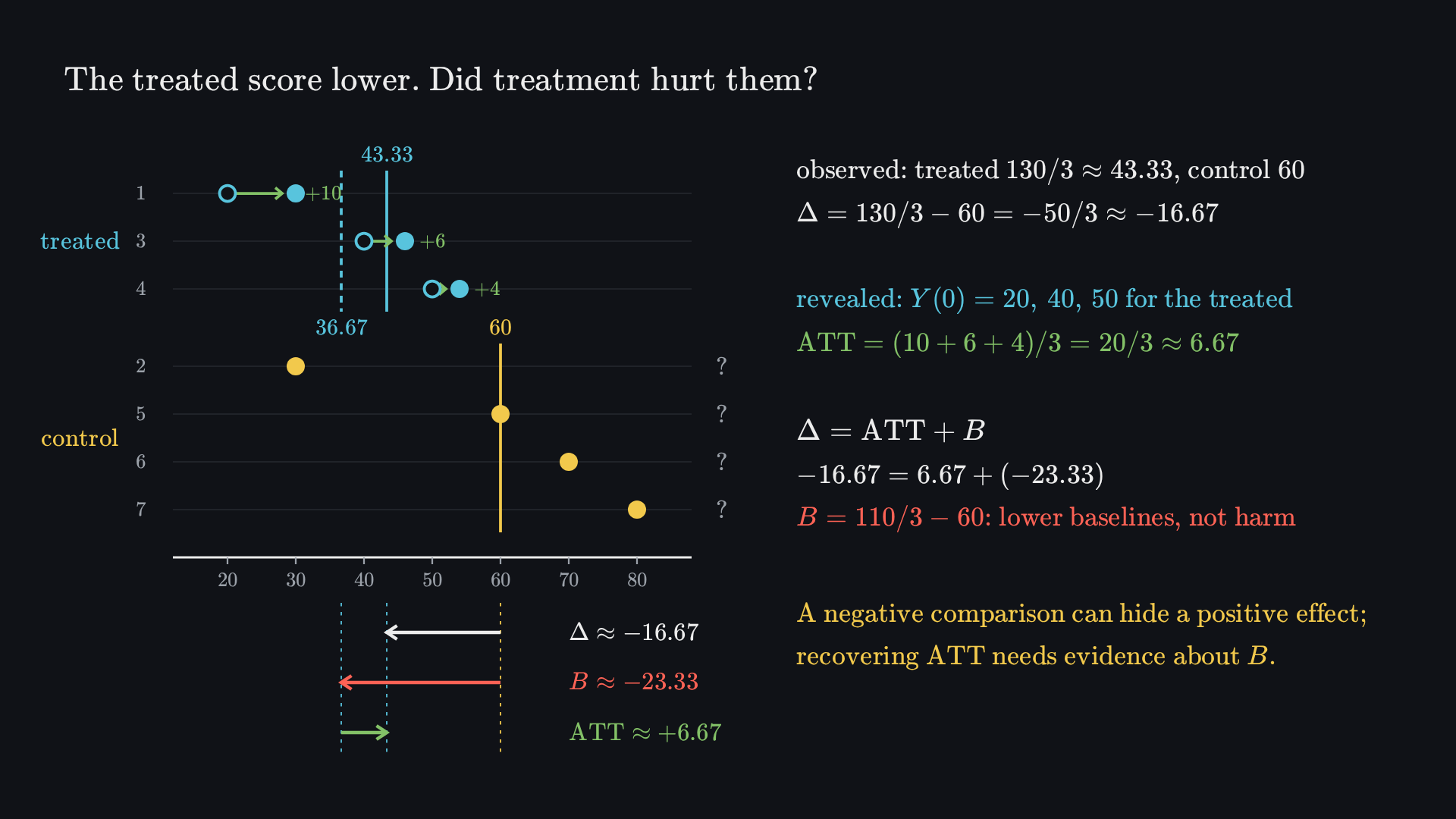
Before playing, predict: the treated group scores 16.67 points below the controls. Does that mean treatment hurt them?The animation’s final frame. Its numbered steps describe how the picture is built.
Observed outcomes only: the treated average 130/3≈43.33 and the controls 60. The comparison Δ=−50/3≈−16.67 makes treatment look harmful.
This toy model also supplies the treated people’s missing no-treatment outcomes, 20,40 and 50. Every one of them gains: ATT=(10+6+4)/3=20/3≈6.67.
The comparison splits as Δ=ATT+B:−16.67=6.67+(−23.33). The selection term B=110/3−60 says the treated would have scored lower anyway.
A negative observed difference is compatible with a positive effect. Recovering ATT needs evidence about B, which the observed outcomes alone cannot give.
ATT
Selection bias
Observed difference
6
−10
−4
The negative observed difference is compatible with a positive ATT. To identify ATT from it, we need evidence about the selection term.
Change the selection term while keeping the hypothetical treatment effect fixed. Predict when the observed comparison changes sign.
5.2.3Two earnings comparisons with different selection mechanisms
A university earnings premium
Suppose, as a lecture illustration, graduates of university O earn £4,000 more than graduates of university X at a stated follow-up date. That observed difference equals ATT plus selection bias for the population and treatment definition used. If the O group would have earned more even at X, B>0, so ATT<£4,000. For example, B=£3,000 would imply ATT £1,000. The observed premium alone does not establish either amount or justify a causal claim about tuition.
A negative training comparison
Use the illustrative difference −£8.80 per week from the training example. If participant selection contributes −£12, the implied ATT is −8.80−(−12)=£3.20 per week. The same negative comparison would suggest harm if selection were zero. These numbers illustrate the decomposition; they are not a verified evaluation of a historical programme.
Selection on gains and selection on baseline outcomes need distinction. People may choose treatment because they expect a large benefit, producing ATT different from ATE. The bias term in this particular identity concerns the untreated baseline Y(0). A claim about selection on gains alone does not determine its sign.
5.2.4Recover an effect only when the bias term is justified
1. Compatible explanations
An observed difference is 12. Give two compatible decompositions, one with an ATT of 5, one with an ATT of 15.
Solution
For ATT 5, selection bias must be 12−5=7. For ATT 15, it must be 12−15=−3. Both satisfy the identity. Observing the difference alone cannot choose between them.
2. Population data do not fill counterfactual cells
Every person in a country appears in the dataset. Does this make the observed treatment-group difference causal?
Solution
No. Complete population observation removes the need to estimate the observed group means from a sample. It still reveals only one potential outcome per person. A design or substantive identification assumption is needed to connect the control mean with the treated group's missing no-treatment mean.
5.3 Random assignment and imperfect take-up
What randomization identifies, and why chance imbalance remains
5.3.1Randomize assignment, not the outcome
Random assignment makes the assignment mechanism independent of potential outcomes. In a population model with treatment assigned with the same positive probability to every unit, write
D⊥⊥{Y(0),Y(1)}.
Read the symbol as “D is independent of the pair of potential outcomes.” This does not say observed Y is independent of D. A treatment effect is precisely a way in which assignment can change the observed outcome.
Independence for the untreated world.E[Y(0)∣D=1]=E[Y(0)∣D=0]=E[Y(0)].
Selection term. These equal means make B=0, so the observed population comparison equals ATT.
Independence for both worlds. Also E[Y(1)∣D=1]=E[Y(1)]. Therefore the same comparison equals ATE; in this population model ATT equals ATE.
The mechanism supports comparisons of both observed and unobserved baseline characteristics in expectation. It does not require measuring every cause of the outcome to remove assignment selection.
5.3.2Balanced in expectation is not exactly balanced in every allocation
A realised experiment contains finitely many people. Some random allocations put more high-baseline units in treatment than in control. In a finite-population experiment with a fixed number assigned to each group, the difference in observed means is unbiased for the finite-population ATE over the assignment distribution. It is not necessarily equal to that ATE in the allocation actually obtained.
For the seven-person model, fix three treated units and enumerate the (37)=35 possible complete random assignments. Each allocation has probability 1/35. Potential outcomes stay fixed while the observed cells and group means change. Averaging the difference over all allocations recovers 34/7; a particular allocation can be far from it. With heterogeneous effects, the ATT among the people actually assigned can also differ from the full-population ATE.
Across all 35 equally likely assignments of three treated units, the average difference is 34/7≈4.86. For the initial assignment {1,3,4}, it is −50/3≈−16.67. Randomization removes systematic assignment selection, not every realised baseline imbalance.
This is an exact enumeration of a stated toy design. It separates a single realised comparison from its assignment expectation; it is not a proof that an observational assignment was random.
After the design establishes a causal target, inference quantifies chance variation. The interval chapters explain how standard errors depend on design; matched, clustered or stratified randomization can require methods beyond an independent two-group formula.
5.3.3An offer and treatment received are different variables
Let Z be randomized assignment to an offer and D actual treatment received. Non-compliance means some people offered treatment do not take it. Contamination means some assigned to control obtain it. Both can make received treatment depend on characteristics or potential outcomes.
Comparing people by their received treatment generally forfeits the randomization argument. Comparing them by their randomized offer preserves an intention-to-treat contrast, provided outcomes are observed appropriately and the assignment design is maintained:
ITT=E[Y∣Z=1]−E[Y∣Z=0].
ITT answers the effect of assigning the offer, including take-up under that policy. It is not automatically the effect of receipt. If the offer changes receipt and has no other outcome pathway, stronger assumptions can identify a treatment effect for compliers. The instrumental-variable chapter explains why that effect can be local rather than the ATE.
Differential attrition is another issue: randomized assignment does not ensure that the observed-outcome subset remains comparable. Report take-up and missing outcomes by original assignment group, and explain how each alters the target or identification argument.
5.3.4State what was randomized
1. Assignment versus receipt
An offer is randomized, but more motivated people are more likely to accept. Which comparison inherits the randomization: offered versus not offered, or accepted versus not accepted?
Solution
Offered versus not offered inherits it and targets ITT for the offer. Accepted versus not accepted can contain selection on motivation. A received-treatment effect needs further assumptions and an appropriate design analysis.
2. Chance imbalance
A randomized trial's treated group happens to have a higher baseline mean. Does that fact alone prove randomization failed?
Solution
No. A finite random allocation can be imbalanced by chance. Audit the assignment mechanism and analyse it using its stated design. Conversely, a balanced-looking observational sample does not establish random assignment of unobserved potential outcomes.
5.4 Validity, natural experiments and design
A causal interpretation depends on the mechanism and the target
5.4.1Internal and external validity ask different questions
Internal validity concerns whether the study credibly identifies its stated effect for the units and treatment actually studied. External validity concerns whether that result transports to another target population, setting, implementation or time horizon. Good random assignment can support the first without establishing the second.
Different people, institutions, treatment versions, scale and follow-up.
Participants may change behaviour because they are being observed, sometimes called a Hawthorne effect. Expectations about receiving treatment can also affect outcomes, often discussed as placebo effects. Neither label establishes a universal effect size. Define the comparison: if observation and expectations differ between arms, a contrast may include these components; blinding or an appropriate control can help separate them.
A short study may observe an immediate surrogate rather than the long-term outcome relevant to policy. A biomarker, exam score or short-term employment status is not automatically a complete substitute for later health, learning or earnings. Repeating studies across settings can help identify which circumstances matter, but does not mechanically guarantee transport.
5.4.2Changing scale can change the intervention
The simple potential outcome Yi(d) holds others' assignments implicit. If one person's treatment affects neighbours or coworkers, specify outcomes such as Yi(di,d−i). A small programme and a universal policy then generate different surrounding assignments. Direct effects on recipients and indirect effects on others are different targets.
For a hypothetical preventive intervention, protecting one participant and reducing exposure among untreated neighbours would be two distinct pathways. For a training programme, reallocating a few jobs can have a different effect from increasing everyone's skills. These illustrations explain why effects at trial scale need not equal effects after economy-wide or community-wide adoption; they do not supply medical efficacy claims or policy estimates.
5.4.3External events need an identification argument
When researchers cannot randomize, external events or institutions can create useful treatment variation. A natural experiment uses variation arising outside researcher control; a quasi-experimental design attempts to build a credible comparison from a mechanism that resembles random allocation in the relevant respect. The terminology alone does not validate a design.
Consider studying neighbourhood relocation after a storm or landslip. Destruction might induce some households to move. But hazard exposure may vary with location, building quality or poverty, and the disaster can affect income directly through injury, asset loss or disruption. To interpret a relocation contrast, examine baseline comparability, other outcome pathways and who relocates. An event's unpredictability to residents does not by itself make its consequences independent of potential outcomes.
Name the source of variation. What changed assignment, eligibility or treatment intensity?
State the comparison. Which units would be comparable under the assignment rule?
Exclude competing pathways. Could the event affect the outcome other than through the treatment being studied?
Define the local target. Which units and margin of treatment change does the design identify?
5.4.4A threshold rule creates a useful design opportunity
Angrist and Lavy's 1999 study used an institutional class-size rule as a source of variation. Under the illustrative rule, a grade's enrolment n is divided into enough classes to keep each at no more than 40. The predicted average class size is
q(n)=⌈n/40⌉n.
The ceiling symbol means “round up to the next integer.” At n=40, one class has size 40; at n=41, two classes average 20.5. Enrolment changes smoothly by one pupil while predicted class size jumps. Compare schools near a threshold, with a credible argument about other changes at that cutoff. Actual class sizes need not follow the rule perfectly, so the rule can provide an instrument rather than a perfectly assigned treatment.
The historical study and data periods are described in the authors' working-paper record. The expression here illustrates the mechanism, not a current description of all school policies. A discontinuity is useful only if other outcome determinants do not change discontinuously at the same threshold and units cannot sort in a way that defeats the comparison.
5.4.5Examine the design rather than its label
1. A relocation comparison
Households whose homes flood are compared with households whose homes do not. Why is “the weather was random” insufficient to identify the effect of moving?
Solution
Exposure can depend on location and housing, and flooding can affect outcomes through routes other than relocation. We need an assignment/comparability argument and an account of these direct pathways; random weather does not automatically randomize moving alone.
2. Calculate the threshold change
Calculate predicted class size for enrolment 80 and 81 under the rule above.
Solution
At 80, ⌈80/40⌉=2, so q(80)=40.
At 81, ⌈81/40⌉=3, so q(81)=27.
The predicted average drops by 13. This design-induced contrast is not itself an estimate of a test-score effect.
5.5 Conditional independence and overlap
Compare like with like, then average for the right population
5.5.1What conditioning is assumed to remove
Suppose we observe pre-treatment covariates X, such as prior attainment, age or work history. X may be a vector even when we use a single letter. Conditional independence, also called unconfoundedness in this setting, assumes
D⊥⊥{Y(0),Y(1)}∣X.
Within a fixed covariate group, assignment is independent of the pair of potential outcomes. This says selection on the recorded covariates accounts for the remaining systematic assignment differences relevant to those outcomes. It does not say that potential outcomes are constant within a group, or that adjusting for any long list of variables must make the assumption true.
Write md(x)=E[Y∣D=d,X=x], the observed mean for assignment group d in covariate group x. Consistency and conditional independence imply, wherever both assignment groups exist,
m1(x)m0(x)=E[Y(1)∣X=x],=E[Y(0)∣X=x].
The within-group causal contrast is τ(x)=m1(x)−m0(x). To see why, repeat the selection-bias decomposition holding X=x fixed: conditional independence makes the within-group untreated baseline difference zero. It also equates treated and full-group average effects at that value of x.
5.5.2ATE and ATT use different covariate weights
Knowing all the within-group effects is not enough to select a population target. For a discrete covariate, the law of iterated expectations gives
ATE=x∑τ(x)P(X=x),ATT=x∑[τ(x)×P(X=x∣D=1)].
ATE uses the whole target population's covariate distribution. ATT uses the covariate distribution of treated people. Equal within-group identification does not make these aggregate averages equal when effects and group composition vary. A simple average over cells would assign equal weight to cells regardless of their population shares.
For a continuous covariate, replace sums by integration against the relevant distribution: ATE=∫τ(x)fX(x)dx, while ATT uses fX∣D=1(x). These densities describe the target weights, not a different conditional treatment effect.
A two-cell example
In a hypothetical population, half have X=0 and half X=1. Treatment probabilities are 0.2 and 0.8, respectively. Let m0(0)=10, m1(0)=12, m0(1)=20, m1(1)=26. Assume CIA for this constructed example. Effects are 2 and 6.
Total treatment probability.P(D=1)=0.5(0.2)+0.5(0.8)=0.5.
Treated covariate weights. By conditional probability, P(X=0∣D=1)=0.1/0.5=0.2; the other weight is 0.8.
ATE.0.5(2)+0.5(6)=4.
ATT.0.2(2)+0.8(6)=5.2.
Raw difference. Treated mean is 0.2(12)+0.8(26)=23.2; control mean is 0.8(10)+0.2(20)=12. The difference 11.2 contains ATT 5.2 plus baseline selection 6.
Covariate
Population share
Effect
Treated share
X=0
0.5
2
0.2
X=1
0.5
6
0.8
ATE 4, ATT 5.2, raw comparison 11.2. The model assumes within-cell comparability; the calculations do not establish it from data.
Change treatment selection across the two covariate groups. Their causal effects remain fixed; treated-group weights and the unadjusted comparison change.
5.5.3Common support is a separate requirement
Define the propensity score e(x)=P(D=1∣X=x), the treatment probability at a covariate value. For ATE identification by comparing conditional means, require
0<e(x)<1
throughout the target covariate support, apart from sets of probability zero. If all units with a particular covariate profile are treated, no untreated mean at that profile is observed. If all are untreated, the treated mean is missing. A fitted prediction does not turn a missing comparison into an observed one: it adds extrapolation assumptions.
ATT needs an untreated comparison over the covariate profiles present among treated people. One may instead restrict the target to a region of common support, but then the estimand is an effect for that restricted population. Report this change rather than continuing to call the result the unrestricted ATE.
In samples, even positive population overlap may provide few comparable observations. This is an estimation problem layered on top of identification. A model may smooth across nearby values, but smoothness, functional form and uncertainty then matter.
5.5.4Why fine adjustment rapidly produces sparse cells
Consider an explicitly uniform hypothetical dataset of 100 points in a k-dimensional unit cube. A cell with side h in every dimension occupies fraction hk of the cube. The expected count is therefore 100hk, provided the cell lies wholly inside the support.
Dimensions k
Expected count, h=0.2
1
20
2
4
3
0.8
4
0.16
5
0.032
For five dimensions, obtaining an expected total count of five requires
100h5h=5,=(0.05)1/5≈0.5493.
The cell spans more than half the range of each variable. It still provides only an expected total of five observations, not five in each assignment group. This calculation illustrates the curse of dimensionality under uniformity; it is not a prediction for every real dataset. Nonuniform densities, boundaries and treatment selection can make particular cells more or less populated.
5.5.5An adjusted comparison is only as credible as its adjustment argument
A historical application compares military applicants who enlisted with applicants who did not, using recorded screening characteristics. Angrist's 1998 paper includes a matching/regression strategy as well as an instrumental-variable strategy; see the author's paper record. Here the important identification question is whether unmeasured factors behind the final enlistment decision also predict potential earnings.
For example, persistence or reliable attendance might affect both completion of enlistment and earnings without service. If the covariates do not account for this mechanism, holding recorded variables fixed does not remove the selection problem. Neither the number of controls nor similar observed means directly tests independence involving missing potential outcomes.
Choose covariates using their place in the assignment and outcome mechanism. Relevant pre-treatment confounders can help. Variables caused by treatment can remove part of the effect or introduce selection. Even a pre-treatment variable can be a harmful collider in some causal structures, so timing alone is not a complete rule. The next chapter shows why “control for everything” is not a sound strategy.
5.5.6Check weights, overlap and credibility separately
1. Different target weights
Two strata have effects 3 and 9. Population weights are 0.7,0.3; treated weights are 0.2,0.8. Under within-stratum identification, find ATE and ATT.
Solution
ATE is 0.7(3)+0.3(9)=4.8. ATT is 0.2(3)+0.8(9)=7.8. Both use the same stratum effects; they average over different target populations.
2. No control group at a covariate value
Everyone with X=1 is treated. CIA is assumed. Can a treated-minus-untreated conditional mean comparison identify τ(1) from the observed distribution?
Solution
No. CIA does not supply the missing observed untreated mean at X=1. Common support fails there. Extrapolation or another identification strategy needs additional assumptions, or the target must be restricted.
5.6 Composition, pay gaps and bad controls
An adjusted difference changes the question and can change the comparison
5.6.1A descriptive pay gap is a defined statistic
The dated ONS 2021 bulletin reports UK median hourly-pay gaps excluding overtime: 7.9% for full-time employee jobs, −2.7% for part-time jobs and 15.4% overall. These historical figures were provisional. The achieved ASHE sample was about 140,000, smaller than before the pandemic, with greater uncertainty. Full-time meant more than 30 paid hours weekly, or at least 25 for teaching professions.
The statistic compares pay across jobs; it is not a matched comparison of people doing the same job. The release also reports larger gaps for older and higher-paid groups. These describe distributions, not a causal effect of a specified intervention. A median gap is computed as the difference in group medians divided by the men's median.
Crucially, a pooled median is not a weighted average of subgroup medians. The law of iterated expectations is a statement about means. Do not use it to reconstruct these published median gaps. Even for means, the male and female subgroup weights can differ, and a ratio of means is not generally an average of subgroup ratios.
5.6.2Use a mean illustration to see the composition mechanism
Retain the lecture's rounded pay numbers as an explicitly hypothetical two-stratum mean model. This example is useful for understanding composition; it is separate from the official median calculation.
Stratum
Men's mean
Women's mean
Share of men
Share of women
Full-time
14.81
13.64
0.85
0.58
Part-time
9.07
9.31
0.15
0.42
Pay is in pounds per hour. Apply each group's own weights:
Within full-time jobs it is about 7.90%; within part-time jobs it is about −2.65%. The aggregate exceeds both because women have a larger share in the lower-paid stratum. There is no contradiction: different mixture weights define the overall populations. The rounded inputs do not reproduce 15.4%, and we do not replace exact arithmetic with that published figure.
Different compositions change the aggregate mean
Filled marker: men. Open marker: women. Horizontal axis: hourly mean pay in pounds in the illustrative model.
The aggregate separation can exceed the separation within either employment stratum because each group has different full-time and part-time weights. The chart uses hypothetical means and the stated weights; it does not reconstruct the published ONS medians.
If both groups instead have full-time share 0.85, the female mean becomes 12.9905. The resulting overall mean gap is about 6.87%. Standardizing composition answers a different descriptive question; it is not automatically causal adjustment.
Change the mixture shares while holding all four within-stratum means fixed. The aggregate gap moves even though none of the stratum pay means changes.
5.6.3What Simpson-type reversals reveal
A pooled comparison can be much larger than, smaller than or opposite in sign to every within-group comparison when group composition differs. This is the mechanism commonly discussed under Simpson's paradox. It appears in comparisons of admissions across departments or treatment outcomes across case-severity groups: a group can concentrate in harder-to-enter departments or more difficult cases.
To diagnose the pattern, display the subgroup outcomes and each comparison group's subgroup weights. Do not pick the pooled or adjusted result merely because it is more favourable to a claim. Decide which target and comparison the question requires. A decomposition explains an arithmetic pattern, while a causal interpretation requires an account of why the conditioning variable belongs in the design.
If occupation is partly an outcome of barriers, preferences, past opportunities or the treatment under study, conditioning on occupation can remove a relevant pathway and compare differently selected people. A within-job descriptive gap can be useful for its own stated purpose without identifying the total effect of a broader access intervention.
5.6.4A confounder and an outcome are different control candidates
A pre-treatment common cause
Here X influences treatment and outcome. Under an appropriate model, conditioning on it can address this confounding pathway.
Selection through an outcome
Here W is caused by D and U. Holding W fixed can associate D with U, which also predicts Y, while removing a pathway through W.
Arrows express hypothesized causal directions, not estimated correlations. The second diagram contains D→W←U, a collider at W. Among people who reach a selected occupation, those facing a more restrictive access route may have different underlying characteristics. Conditioning can therefore create a comparison that was absent before selection. These graphs are stated toy mechanisms; deciding the appropriate graph is substantive work.
5.6.5Two potential occupations create four types
Extend the potential-outcomes model with W(0) and W(1), potential occupation indicators under two treatment states; 1 denotes a professional job. Observed occupation follows
W=(1−D)W(0)+DW(1).
Type
W(0)
W(1)
Professional under both states
1
1
Professional only under state 0
1
0
Professional only under state 1
0
1
Professional under neither state
0
0
Professional workers observed in state 1 belong to {W(1)=1}; those in state 0 belong to {W(0)=1}. These need not be the same types of people. This remains true even under a toy assumption that assignment D is jointly independent of all potential earnings and occupations.
The lecture uses female/male labels to motivate differential access. For a real causal study, a recorded demographic attribute alone does not fully specify an intervention. One might instead define changes in perceived classification, hiring treatment or access rules, specifying the pathways and treatment versions of interest. The two-state model here shows a selection mechanism; it does not estimate a causal effect of sex or establish that any particular access mechanism operates in the population.
5.6.6Equal observed pay within a profession can mask a negative effect
Under the stated joint-independence toy assumption, the observed professional contrast can be written without conditioning further on D:
ΔW=E[Y(1)∣W(1)=1]−E[Y(0)∣W(0)=1].
Add and subtract E[Y(0)∣W(1)=1]. This produces a causal contrast for the fixed group that would be professional under state 1, plus a composition difference between the two potential professional groups:
The reference group stays W(1)=1 in both terms of τW. Calling it an unrestricted ATE would be wrong. Removing D from these conditional means requires joint independence involving earnings and occupation; separate pairwise independence statements are not sufficient in general.
A fully specified counterexample
Imagine the following potential population, with assignment independent of type. Earnings are invented units.
Type share
W(0)
W(1)
Y(0)
Y(1)
0.50
1
1
100
85
0.30
1
0
60
45
0.20
0
0
40
25
Individual effects. Every type has Y(1)−Y(0)=−15.
Professionals in state 1. Only the first type qualifies, so their observed mean is 85, and their counterfactual state-0 mean would be 100.
Professionals in state 0. The first two types qualify. Their mean is [0.5(100)+0.3(60)]/0.8=85.
Observed within-profession gap. It is 85−85=0, yet τW=−15 and BW=100−85=15.
The example establishes logical compatibility: zero observed within-profession difference does not rule out a negative causal contrast when composition changes. It does not establish the direction or size of a real-world bias. A total effect, a direct effect holding occupation fixed and a comparison among always-professional types are different estimands and require different assumptions.
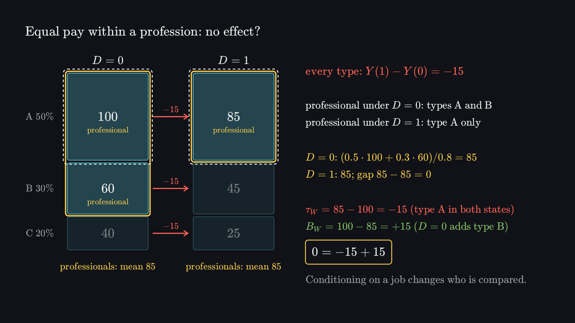
Before playing, predict: among professionals, both groups earn 85. Does that show the treatment has no effect on earnings?The animation’s final frame. Its numbered steps describe how the picture is built.
Three types of people, with shares 50%,30% and 20%, have earnings under both states. Every type earns 15 less under D=1.
Occupation depends on the state: types A and B are professionals under D=0, but only type A under D=1.
Compare professionals only: (0.5⋅100+0.3⋅60)/0.8=85 under D=0 and 85 under D=1. The within-profession gap is 0.
For the same people, type A, the effect is τW=85−100=−15. The D=0 professionals also include lower-paid type B, so BW=100−85=+15. The zero gap is −15+15: conditioning on a job changes who is compared.
5.6.7Separate descriptive standardization from causal identification
1. Can LIE average medians?
Two strata have published median pay gaps. Can their weighted average be used to calculate the pooled median pay gap?
Solution
No. A pooled median depends on the entire mixture distribution and is not generally a weighted average of subgroup medians. LIE concerns means. Even a mean gap needs each group's own stratum weights and the appropriate denominator.
2. A selected professional group
In the three-type toy model, why does the professional comparison equal zero while every person's treatment effect equals −15?
Solution
The professional sets differ by state. State 1 professionals all have untreated potential earnings 100; state 0 professionals include a lower-baseline type, producing untreated mean 85. Selection of +15 offsets the causal contrast of −15. The two observed means therefore compare different mixtures.
5.7 Offers, instruments and local effects
A supplementary bridge from imperfect take-up to LATE
5.7.1Why an instrument changes the treatment comparison
This chapter supplies an additional derivation of local average treatment effects, a topic named in the introductory outline. The mechanism and conditions follow the framework associated with Imbens and Angrist's work. An instrument Z changes the probability of receiving treatment D. A randomized offer is a useful example: assignment is known, while receipt may still be chosen.
Define D(1) and D(0), potential receipt under an offer and no offer. Under exclusion, the offer has no effect on the outcome except through receipt, so the outcome under assignment is Y(D(Z)). This is a substantive restriction: information, expectations or alternative services caused by the offer could violate it.
In addition to exclusion, use four conditions for the elementary binary-instrument result: joint independence of Z from all potential receipt and outcome variables; positive probabilities of both assignment states; a nonzero effect of assignment on receipt; and monotonicity D(1)≥D(0). Also require the defined treatment versions, consistency and no interference used in the preceding model.
5.7.2Compliance types and the role of monotonicity
Type
D(0)
D(1)
Response to offer
Never-taker
0
0
No receipt under either state.
Complier
0
1
Receipt changes with the offer.
Always-taker
1
1
Receipt under either state.
Defier
1
0
Receipt changes against the offer.
Monotonicity rules out defiers for this instrument and treatment direction. It does not say all people comply, that effects are positive, or that the complier effect equals the population average. Under independence and no defiers, the difference in receipt rates is the population share of compliers:
πC=E[D∣Z=1]−E[D∣Z=0].
Always-takers and never-takers keep the same receipt state when the offer changes. Under exclusion, they contribute no outcome change caused by the offer. Compliers switch from Y(0) to Y(1).
5.7.3Deriving the Wald ratio
Outcome effect of the offer. Independence identifies the assignment contrast as the expected change in Y(D(Z)).
Split by compliance type. Under exclusion, only compliers change outcomes when assignment changes; monotonicity removes the oppositely switching type.
Weight their effect. The outcome contrast is therefore πCE[Y(1)−Y(0)∣C].
Remove the complier share. Divide by the nonzero receipt contrast πC.
Read LATE as “local average treatment effect.” It is local to the people whose receipt changes under this particular instrument. Another offer, eligibility threshold or encouragement may move different people and identify another local average. With heterogeneous effects, LATE, ATE and ATT can all differ.
A numerical offer example
In a hypothetical valid-instrument model, 20% are always-takers, 50% compliers and 30% never-takers. Receipt rises from 0.20 without the offer to 0.70 with it. Suppose the outcome assignment difference is 3 points. The complier effect is 3/(0.70−0.20)=6 points. Effects for always-takers and never-takers are not recovered from this comparison alone.
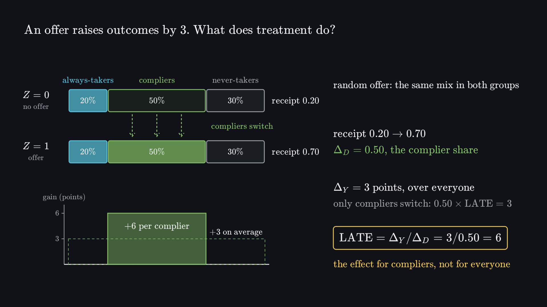
Before playing, predict: a random offer raises average outcomes by 3 points and moves receipt from 20% to 70%. How large is the treatment’s effect for those who switch?The animation’s final frame. Its numbered steps describe how the picture is built.
A randomised offer gives both groups the same mix of types: 20% always-takers, 50% compliers and 30% never-takers.
Receipt rises from 0.20 without the offer to 0.70 with it. Only compliers switch, so ΔD=0.50 is the complier share.
The offer raises the average outcome by ΔY=3 points. If the offer affects outcomes only through receipt, the whole gain comes from the compliers: 0.50×LATE=3.
So LATE=ΔY/ΔD=3/0.50=6 points, the effect for compliers. It is not, by itself, the effect for always-takers, never-takers or everyone.
5.7.4A larger receipt effect is not a universal effect
1. Calculate and name the target
Offer assignment changes receipt from 0.10 to 0.40, and mean outcomes by 1.2. Under the binary-instrument assumptions, find and interpret the effect.
Solution
First stage.ΔD=0.40−0.10=0.30.
Ratio.LATE=1.2/0.30=4.
Target. This is an average effect of 4 outcome units among compliers induced by this instrument; it is not automatically ATE or ATT.
2. An offer changes expectations
A randomized offer improves outcomes through reassurance even for people who never receive the programme. Which key assumption is threatened?
Solution
Exclusion. The offer now has a direct outcome pathway besides receipt. The simple decomposition in which only switching recipients contribute no longer holds, so the ratio need not identify the complier receipt effect.
5.7.5Bring identification and inference together
Before reporting a causal estimate, state the intervention, target population, outcome and time; draw or describe the assignment mechanism; name the identifying conditions; check which comparisons have support; and then select inference appropriate to the design. A confidence interval describes estimation uncertainty under its assumptions. It does not include every possible violation of CIA, exclusion, treatment definition or transport.
The course now joins five distinct tasks: probability defines uncertainty; distributions and moments describe measurements; statistics studies sampling variation; time series accounts for temporal dependence; causal inference determines which comparison can answer an intervention question. Use the distinction between an identity, an assumption and a result under conditions whenever a formula seems to promise more than the design provides.